Week 5 — Bayesian Networks & Causal Bayes Nets第5週 — ベイズネットと因果ベイズネット

Friday, May 29, 20262026年5月29日（金）

Prof. Joseph Austerweilオウステウェイル　ジョセフ教授

Agenda本日の予定

• Your assignment IS a Bayes net皆さんの課題はベイズネットです 0:00
• Two complications + notation2つの拡張 + 記号の確認 0:10
• Chibany Monty Hall + formal definitionチバニーのモンティ・ホール + 正式な定義 0:20
• d-separation + Bayes-Balld分離 + ベイズボール 0:35
• Explaining away説明はがし 1:00
• Break休憩 1:12
• Observation → intervention観測 → 介入 1:22
• The do-operatordo演算子 1:32
• Blicket detectorブリケット検出器 1:47
• Information theory + close情報理論 + まとめ 1:55

~1 min agenda overview. Today’s spine: the Gaussian mixture from Clusters turns out to be a Bayes net you’ve already been doing. We build up to multi- parent networks, name the formal object, then go through d-separation, explaining-away, and the causal Bayes-net machinery (do-operator). Close with 3 info-theory slides connecting back to the collider. No student presenter this week — we have more time per block.

Terminology: four overlapping names用語：重なり合う4つの名前

Before we start — these terms get used loosely, sometimes interchangeably. Here’s the relationship for today:

• Graphical model — umbrella term. Any probabilistic model drawn as a graph. Includes directed (Bayes nets) and undirected (Markov random fields) variants.
• Bayesian network (= directed graphical model = belief network) — a DAG where each node is a random variable and arrows encode conditional dependence. Today’s main object.
• Hierarchical Bayesian model — Week 4’s “priors over priors.” Once drawn as a graph, it’s a Bayes net with at least one extra level of parameter nodes feeding into other parameter nodes. So: every hierarchical Bayesian model is a Bayes net. The reverse isn’t true — a Bayes net without that extra layer (e.g. Monty Hall, which we’ll work through later today) is “flat,” not hierarchical.
• Causal Bayesian network — same DAG, but arrows now mean direct causation. Adds the do-operator (Pearl). Every causal BN is a Bayes net; not every Bayes net is causal.

GMM = hierarchical Bayes ⊂ Bayes net ⊂ graphical model. Causal BN = Bayes net + causal reading.

始める前に — これらの用語は緩く、時には互換的に使われます。今日のための関係：

• グラフィカルモデル — 総称。グラフとして描かれる確率モデル全般。 有向（ベイズネット）と無向（マルコフ確率場）の両方を含む。
• ベイズネット (= 有向グラフィカルモデル = 信念ネットワーク) — DAG で、各ノードが確率変数、矢印が条件付き依存性を表す。今日の主役。
• 階層ベイズモデル — 第4週の「事前分布の上の事前分布」。グラフに描けば、 パラメータノードが別のパラメータノードに流れ込む追加の層 を持つベイズネット。 つまり：階層ベイズモデルはすべてベイズネット。 逆は真ではない — その追加の 層がないベイズネット（例：モンティ・ホール、今日後で扱います）は「フラット」で あり、階層的ではない。
• 因果ベイズネット — 同じDAGだが、矢印は 直接的な因果関係 を意味する。 do演算子（Pearl）が加わる。因果BN はすべてベイズネット；ベイズネットがすべて 因果的なわけではない。

GMM = 階層ベイズ ⊂ ベイズネット ⊂ グラフィカルモデル。因果BN = ベイズネット + 因果的解釈。

~2 min. Set the vocabulary BEFORE the build-up. Two students could otherwise think “Bayesian network” = “the thing with hyperpriors from Week 4” or = “the causal thing we’ll do later.” Lock in the containment relationship now: graphical model ⊃ Bayes net ⊃ hierarchical BN. Causal BN = Bayes net + a specific interpretation of the arrows (and the do-operator). Mention undirected GMs briefly (one sentence) — we won’t cover them today but students should know the umbrella isn’t only DAGs. Reference back to this slide if anyone asks “is X a Bayes net or a hierarchical model?”

Your assignment IS a Bayes net皆さんの課題はベイズネットです

Welcomeようこそ

Week 5 of Human and Machine Learning.

Last week we wrestled with hierarchical Bayes — priors over priors. Right now most of you are mid-Clusters, working out Gaussian mixtures.

Today’s claim: those are the same thing, drawn as a graph.

人間と機械の学習、第5週。

先週は 階層ベイズ — 事前分布の上の事前分布 — に取り組みました。 今は皆さんの多くがクラスタ課題の途中で、ガウス混合モデル を解いていますね。

今日の主張：その2つは同じものを、グラフで描いただけだ、ということです。

30 sec opening. Set up the recognition moment: you’ve been doing this; let’s name it. Don’t pre-empt the punchline — let the GMM-as-DAG slide deliver it.

Chibany’s histogram, drawn differentlyチバニーのヒストグラム、別の描き方で

Remember Chibany’s mystery bentos? Two peaks at 350g and 500g.

In Clusters you’re writing a two-Gaussian mixture as a generative process and computing what each datapoint tells you about which cluster it came from.

Today’s claim: that generative process is a Bayes net. Same model — just drawn. You’ve been doing Bayesian-network inference all week without naming it.

We’ll leave the density and the “which cluster?” formula to your assignment — no spoilers today.

チバニーのミステリー弁当を覚えていますか？350g と 500g の2つのピーク。

クラスタ課題では、2成分ガウス混合を 生成過程 として書き、各データ点が どのクラスタから来たかを計算していますね。

今日の主張：その生成過程は ベイズネットそのもの。同じモデル、ただ図に描いただけ。 皆さんは今週ずっと、名前を付けずにベイズネットの推論をしていたんです。

密度の式と「どのクラスタか？」の式は課題で導出してもらうので、今日はネタバレなし。

~2 min. RECOGNITION slide. NOTE: density formula and responsibility formula are deliberately omitted — they’re Problems 1 & 2 of Clusters, due Friday and not all submitted yet. Set up the “you’ve been doing it” payoff without spoiling the algebra. Lecture flow: name the model conceptually, promise to show it as a graph, deliver via the build-up steps.

The generative process you wrote皆さんが書いた生成過程

In Clusters Problem 2, you wrote the two-Gaussian mixture as:

\[c_n \mid \theta \;\sim\; \mathrm{Bernoulli}(\theta)\] \[x_n \mid \mu_{c(n)},\, \sigma^2_{c(n)} \;\overset{iid}{\sim}\; \mathrm{N}(\mu_{c(n)},\, \sigma^2_{c(n)})\]

Two lines. Each line is one sampling step. Today we’ll show that this generative process is already a Bayes net — we just haven’t drawn it yet.

クラスタの問題2 では、2成分ガウス混合を次のように書きました：

\[c_n \mid \theta \;\sim\; \mathrm{Bernoulli}(\theta)\] \[x_n \mid \mu_{c(n)},\, \sigma^2_{c(n)} \;\overset{iid}{\sim}\; \mathrm{N}(\mu_{c(n)},\, \sigma^2_{c(n)})\]

2行。各行が 1つのサンプリングステップ。今日は、この生成過程が すでにベイズネットである ことを示します — 単にまだ図に描いていないだけ。

~60 sec. Anchor on the exact notation from the assignment. Two lines — emphasize each is one sample step. Then promise the visualization.

Step 1: introduce θステップ1：θを導入

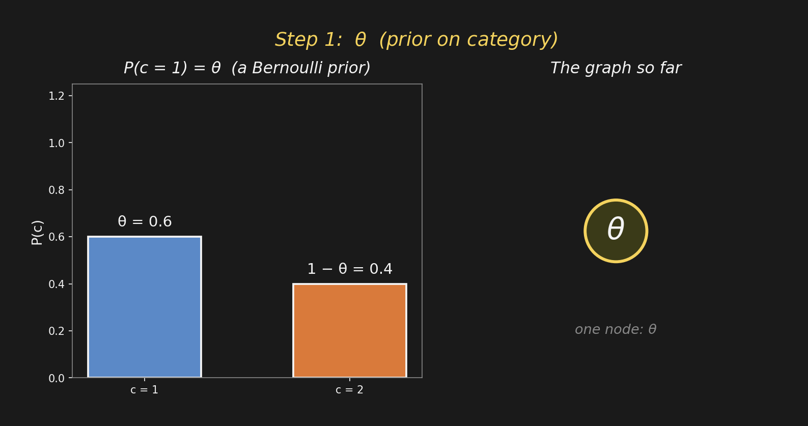
The Bernoulli prior on the left has one parameter, \(\theta\). On the right, \(\theta\) becomes one node of the graph. A node = a random variable (or parameter) in the model.

左のベルヌーイ事前分布にはパラメータ \(\theta\) が1つ。右では、\(\theta\) がグラフの ノード の1つになる。ノード = モデル中の確率変数（またはパラメータ）。

~60 sec. Spend a beat on each panel. Left: theta is a number on [0,1] that sets the bar heights. Right: that same number is a node. Same θ, two pictures.

Step 2: sample \(c_n \sim \mathrm{Bernoulli}(\theta)\)ステップ2：\(c_n \sim \mathrm{Bernoulli}(\theta)\) をサンプル

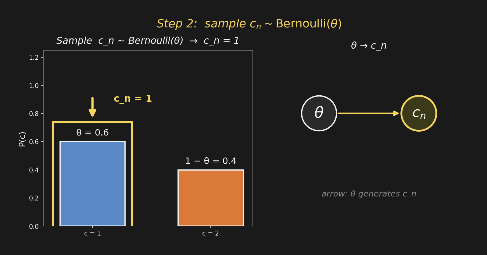
Sampling \(c_n\) flips a θ-weighted coin. Pick category 1 (highlighted bar). On the graph: \(c_n\) becomes a new node, and the line \(c_n \mid \theta \sim \mathrm{Bernoulli}(\theta)\) becomes an arrow from θ to \(c_n\).

Generative-process line ↔︎ arrow in the graph.

\(c_n\) のサンプリングは、θ で重み付けされたコインを振る。カテゴリ1 を選ぶ（黄色いバー）。 グラフの上では： \(c_n\) が新しいノードになり、\(c_n \mid \theta \sim \mathrm{Bernoulli}(\theta)\) という行は θ から \(c_n\) への 矢印 になる。

生成過程の1行 ↔︎ グラフの矢印1本。

~75 sec. THE central pedagogical move. The ‘arrow’ is exactly the conditioning bar in the generative process. Spell this out — “the | in c_n | θ IS the arrow from θ to c_n.”

Step 3: introduce the componentsステップ3：成分を導入

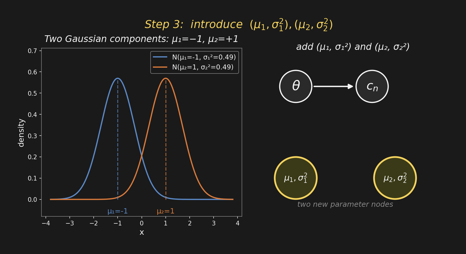
The two Gaussians have parameters \((\mu_1, \sigma_1^2)\) and \((\mu_2, \sigma_2^2)\). On the graph: two new nodes for the parameters — one pair per component.

We’re not yet drawing arrows from these into \(x_n\). That happens in the next step.

2つのガウス分布のパラメータは \((\mu_1, \sigma_1^2)\) と \((\mu_2, \sigma_2^2)\)。グラフの上では： パラメータごとに新しいノード — 成分ごとに1ペア。

まだ \(x_n\) への矢印は描かない。それは次のステップ。

~60 sec. Show two Gaussians at μ=-1 and μ=+1 (exact values from Problem 2). Add parameter nodes but no edges into x yet — keep the build-up tidy.

Step 4: sample \(x_n\), the observationステップ4：観測 \(x_n\) をサンプル

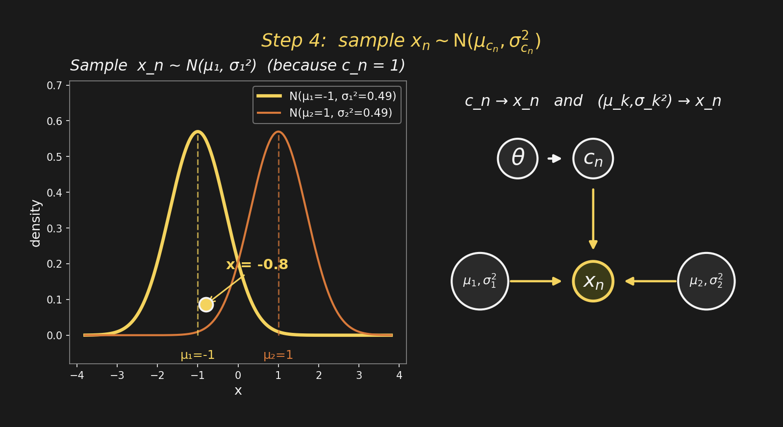
With \(c_n = 1\), we sample \(x_n \sim \mathrm{N}(\mu_1, \sigma_1^2)\) — a point under the highlighted Gaussian. On the graph: \(x_n\) is a new node (shaded — it’s observed), with arrows from \(c_n\) and from each \((\mu_k, \sigma_k^2)\).

The second generative-process line gave us three new arrows at once.

\(c_n = 1\) のとき、\(x_n \sim \mathrm{N}(\mu_1, \sigma_1^2)\) をサンプル — 黄色いガウス分布の下の1点。グラフの上では： \(x_n\) は新しいノード（網掛け = 観測済み）、\(c_n\) と各 \((\mu_k, \sigma_k^2)\) から矢印が入る。

生成過程の2行目で、矢印が3本 一気に加わった。

~75 sec. Shaded x_n = observed convention. Point out: x_n depends on c_n (which Gaussian) AND on (μ_k, σ_k) (the parameters of that Gaussian). Three arrows from one generative-process line.

Step 5: do this N timesステップ5：これを N 回繰り返す

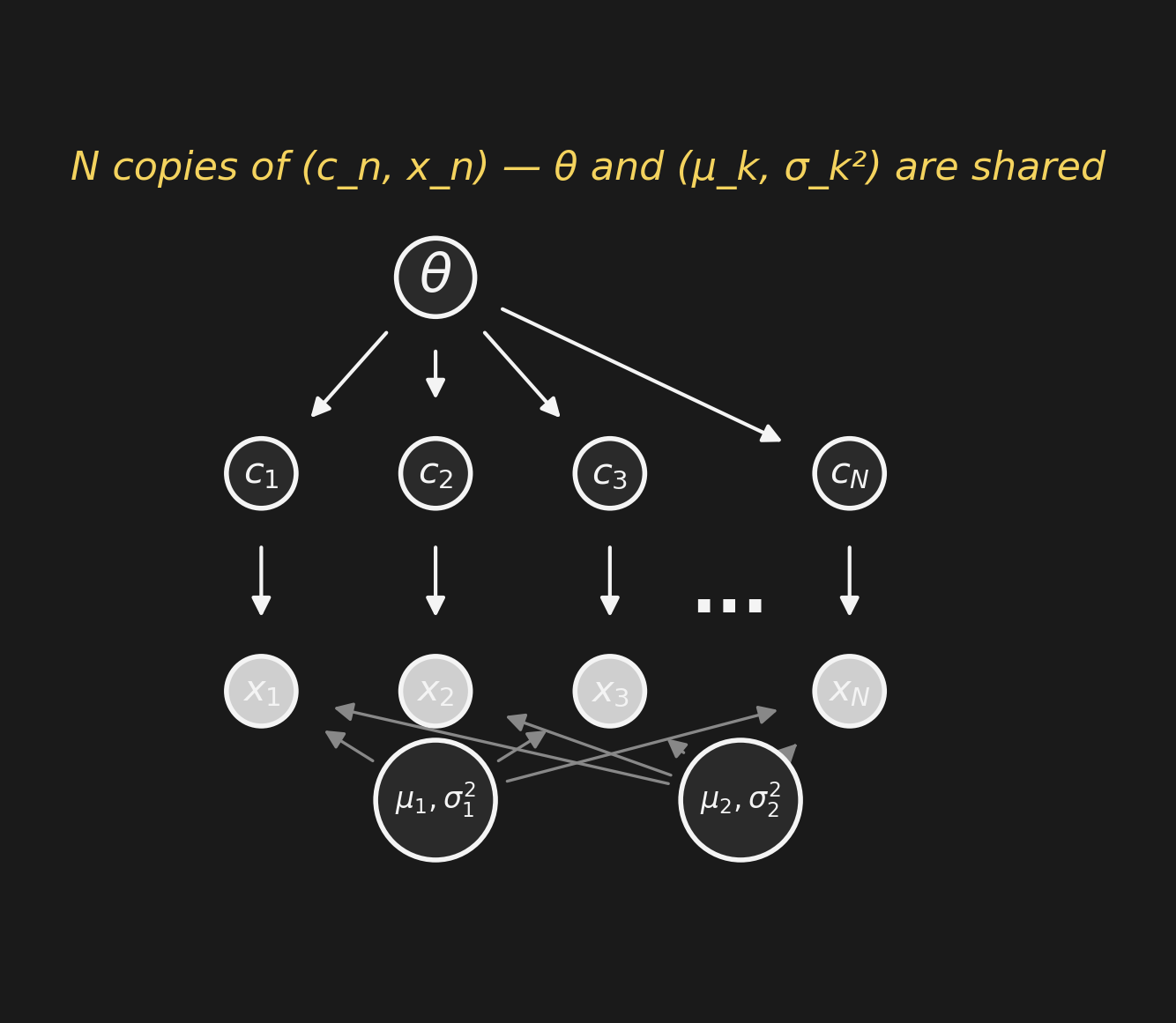
The generative process has \(n = 1, \ldots, N\). Each \(n\) gets its own \((c_n, x_n)\) — but \(\theta\) and the \((\mu_k, \sigma_k^2)\) are shared.

Drawn explicitly, this is an N-fold copy of the same little pattern.

生成過程は \(n = 1, \ldots, N\) にわたる。各 \(n\) に独自の \((c_n, x_n)\) — しかし \(\theta\) と \((\mu_k, \sigma_k^2)\) は 共有される。

明示的に描くと、同じ小さなパターンの N 個のコピー。

~60 sec. Show 3 copies + “…” + the Nth. The shared parameters are drawn once; the per-datum nodes are drawn N times. Set up the plate motivation: this is correct but unwieldy.

Step 6: the plate — a shortcutステップ6：プレート — 略記法

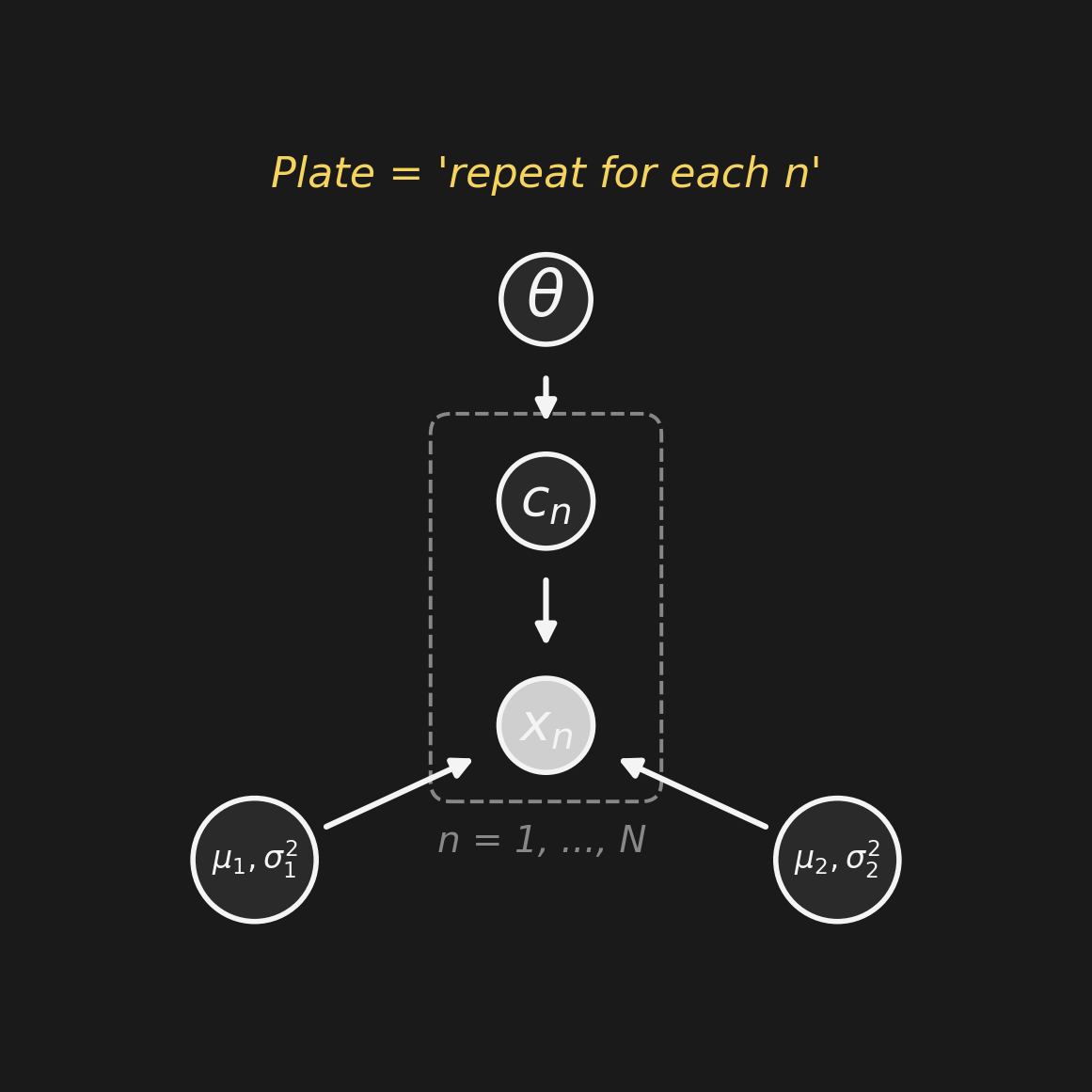
Plate notation: draw the repeating pattern once inside a dashed box, and label the box “\(n = 1, \ldots, N\).” The plate means “copy everything inside, N times.”

Same graph, vastly more compact.

プレート記法： 繰り返しパターンを 1回だけ 破線の箱の中に描き、箱に “\(n = 1, \ldots, N\)” とラベルを付ける。プレートの意味は 「中身を N 回コピー」。

同じグラフ、はるかにコンパクト。

~45 sec. Plate is purely notation — no new content. Just compress the unrolled graph. Bishop, Murphy, Koller all use this.

Step 7: generalize to K componentsステップ7：K成分に一般化

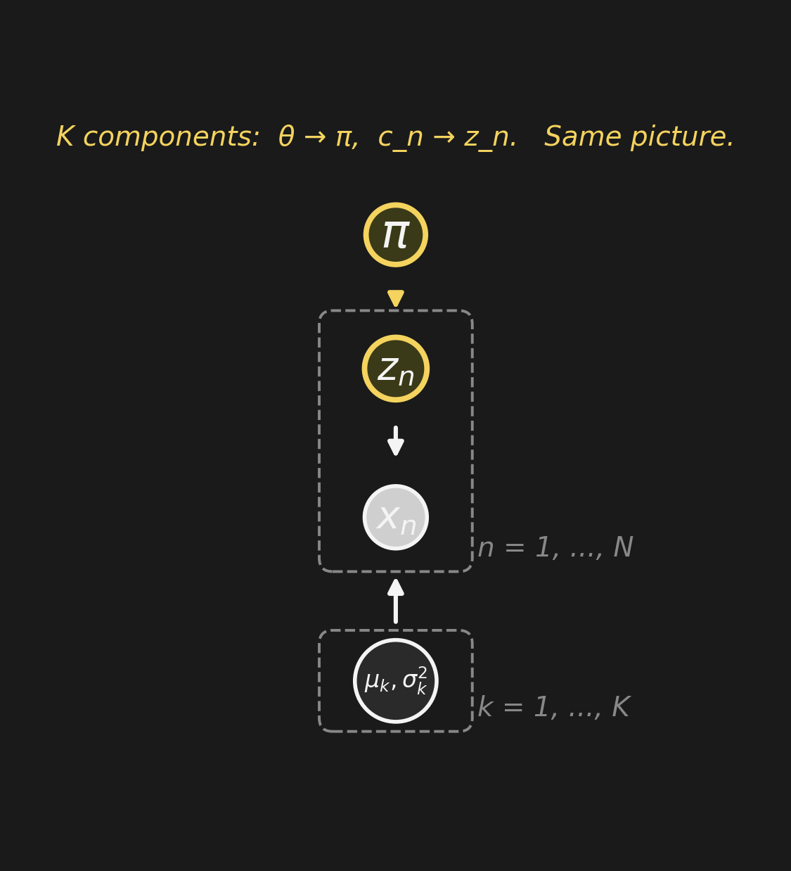
Bernoulli(\(\theta\)) generalizes to Categorical(\(\pi\)) for K components. \(c_n \to z_n\), \(\theta \to \pi\), and \((\mu_k, \sigma_k^2)\) gets a K-plate.

Same picture. Two clusters or two hundred — the graph language stayed put.

Bernoulli(\(\theta\)) は K 成分の場合の Categorical(\(\pi\)) に一般化される。 \(c_n \to z_n\)、\(\theta \to \pi\)、\((\mu_k, \sigma_k^2)\) には K-プレートを付ける。

同じ絵。 2つのクラスタでも200個でも — グラフ言語はそのまま。

The choice of K — DPMM (T3 Ch 6) avoids fixing it. Week 10 picks this up.

~60 sec. Quick generalization. The notation switch (c_n → z_n, θ → π) is just renaming. The K-plate is the new structural piece. DPMM gets the one-line forward pointer.

Reading inference off the graphグラフから推論を読み取る

You’ve now seen the graph. Two things to take away — without writing down the formula (that’s your assignment):

• Down the arrow = generative direction. Sample \(\theta\), then \(c_n\), then \(x_n\).
• Up the arrow = inference direction. Observe \(x_n\), ask which \(c_n\) generated it.

The “which cluster?” calculation you’re doing in Clusters Problem 2 is inference going UP the arrow from \(x_n\) to \(c_n\). Prior → likelihood → posterior, read off the parent–child structure.

We won’t write the formula here — finish the assignment first; we’ll discuss after Friday.

グラフを見たので、2つの要点を持ち帰ってください — 式は書かずに（それは課題）：

• 矢印を下る = 生成方向。\(\theta\) をサンプル、次に \(c_n\)、次に \(x_n\)。
• 矢印を上る = 推論方向。\(x_n\) を観測して、どの \(c_n\) から来たかを問う。

クラスタ課題の問題2 でやっている「どのクラスタか？」の計算は、まさに \(x_n\) から \(c_n\) へ矢印を上る推論。事前 → 尤度 → 事後を、親子構造から読み取る。

式はここでは書きません — まず課題を提出してから、金曜後に解説します。

~75 sec. PAYOFF slide. NOTE: previous version showed the full responsibility formula — REMOVED because that’s Problem 2 of Clusters (due Friday, not all submitted). Keep the conceptual claim (“up the arrow = inference”) without giving away the algebra. Verbal hint to students: “the formula falls out of the graph naturally, but write it yourself — we’ll go over it next class.”

Two complications + notation2つの拡張 + 記号の確認

Where do the priors come from?事前分布はどこから来るのか？

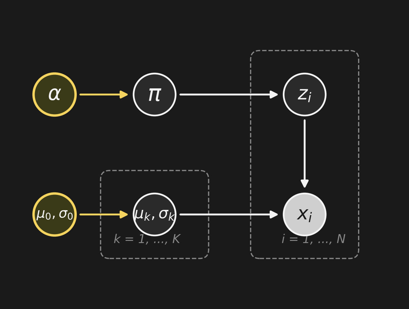
Add a hyperprior: \(\alpha \to \pi\) and \((\mu_0, \sigma_0) \to (\mu_k, \sigma_k)\).

This is exactly Week 4’s hierarchical Bayes, drawn as a graph. The graph language already covered it; we just didn’t have the words yet.

ハイパー事前分布 を追加する：\(\alpha \to \pi\) と \((\mu_0, \sigma_0) \to (\mu_k, \sigma_k)\)。

これは 先週の階層ベイズそのもの を、グラフで描いたものです。 グラフという言語ですでに表現できていたのに、その言葉を持っていなかっただけ。

~90 sec. Connect explicitly to Week 4 — hyperpriors are nodes upstream of priors, the directional edges encode “this generates that’s parameters.” The yellow-highlighted nodes are the additions. Don’t dive into hyperprior inference; the point is just “the picture scales.”

What if there are multiple parents?親ノードが複数ある場合は？

Chibany realizes: the bento (\(B\)) weight depends on more than just which cluster.

• Weather (\(W\)) — hot days mean lighter bentos
• Day of the week (\(D\)) — the cafeteria menu rotates
• Restaurant (\(R\)) — different students come from different places

Multiple causes, one observation. How does the picture handle that?

We’ll use \(W\), \(D\), \(R\), \(B\) as shorthand for these variables from here on.

チバニーは気づきます： 弁当 (\(B\)) の重さは、どのクラスタかだけでは決まらない。

• 天気 (\(W\)) — 暑い日は軽めの弁当
• 曜日 (\(D\)) — カフェテリアのメニューはローテーション
• レストラン (\(R\)) — 学生によって出身地が違う

複数の原因、1つの観測値。 グラフはこれをどう扱う？

以降、これらの変数を \(W\), \(D\), \(R\), \(B\) と略記します。

~60 sec. Set up the multi-parent slide. Stay light here — it’s a question, not yet an answer. The answer is on the next slide.

Chibany’s full bento networkチバニーの完全な弁当ネットワーク

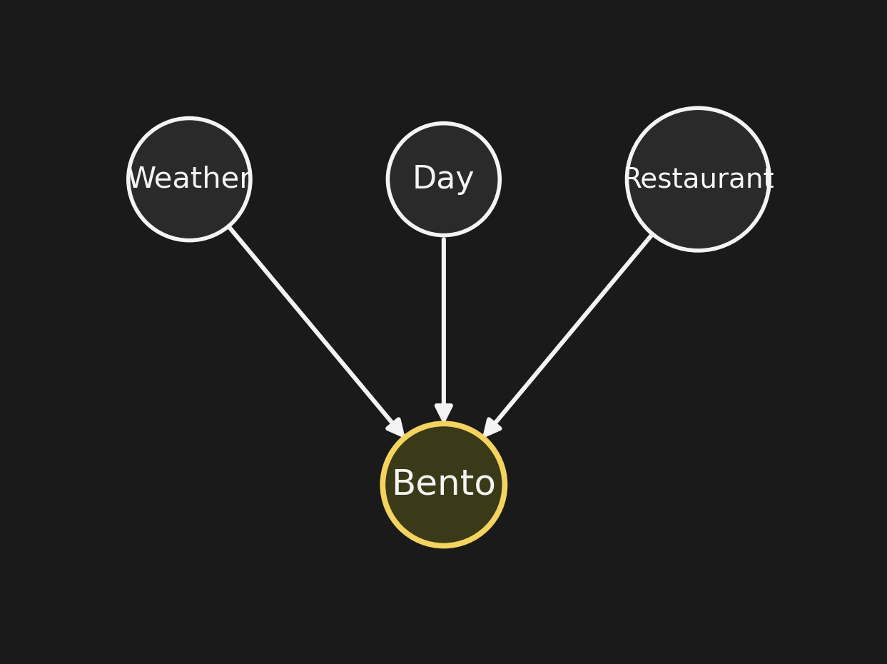
Three parents pointing into Bento. What’s the joint distribution?

3つの親ノードが弁当に向かう。同時分布は何になるか？

~45 sec. Show the graph, pose the question. Let the audience think for a beat before the rule appears next slide. Show-before-tell.

The rule for multiple parents親が複数あるときのルール

Each parent contributes a factor. The joint factorizes as: \[P(W, D, R, B) \;=\; P(W) \, P(D) \, P(R) \, P(B \mid W, D, R)\]

• \(W\), \(D\), \(R\) have no parents → marginals.
• \(B\) has three parents → conditional on all three.

One factor per node, conditioned on that node’s parents. That’s the rule.

各親ノードが因子を1つ提供する。同時分布は次のように因数分解される： \[P(W, D, R, B) \;=\; P(W) \, P(D) \, P(R) \, P(B \mid W, D, R)\]

• \(W\)、\(D\)、\(R\) には親がない → 周辺確率。
• \(B\) には3つの親 → 3つすべて に条件付けられる。

各ノードにつき1つの因子、その親に条件付けられた形で。 これがルールです。

~90 sec. State the rule. Don’t yet name it “the Markov factorization” — that happens in Block 3. Here it’s just shorthand. Note explicitly: nodes without parents are easy (marginals); nodes with many parents need the full CPT.

Notation lock-in記号の確認

Symbols we’ll use:

• \(G = (V, E)\) — a directed acyclic graph (DAG)
• \(\text{Pa}(X)\) — the parents of node \(X\) in \(G\)

使う記号：

• \(G = (V, E)\) — 有向非巡回グラフ (DAG)
• \(\text{Pa}(X)\) — グラフ \(G\) における \(X\) の 親 ノード

Three examples so far:

• GMM: \(\text{Pa}(z_i) = \{\pi\}\), \(\text{Pa}(x_i) = \{z_i\}\)
• GMM + hyperprior: add \(\text{Pa}(\pi) = \{\alpha\}\)
• Bento: \(\text{Pa}(B) = \{W, D, R\}\)

ここまでの3つの例：

• GMM: \(\text{Pa}(z_i) = \{\pi\}\)、\(\text{Pa}(x_i) = \{z_i\}\)
• ハイパー事前を追加: \(\text{Pa}(\pi) = \{\alpha\}\)
• 弁当ネット: \(\text{Pa}(B) = \{W, D, R\}\)

Joint factorizes as: \[P(X_1, \ldots, X_n) = \prod_i P(X_i \mid \text{Pa}(X_i))\]

Same picture, same rule, three problems.

同時分布の因数分解： \[P(X_1, \ldots, X_n) = \prod_i P(X_i \mid \text{Pa}(X_i))\]

同じ絵、同じルール、3つの問題。

~90 sec. This is the C-concession: shorthand notation lock-in, but I’m NOT yet calling the product formula “the Markov factorization.” That’s for Block 3 after Monty Hall lands. Frame this slide as “the shorthand we’ll use next.”

Chibany Monty Hall + formal definitionチバニーのモンティ・ホール + 正式な定義

A new puzzle for Chibanyチバニーへの新しい謎

The cafeteria scenario. Three bento boxes on the counter. Exactly one of them contains tonkatsu (the other two don’t). Chibany picks box 1. The cafeteria worker — who knows which box has the tonkatsu — opens box 3 and reveals: not tonkatsu.

Should Chibany switch to box 2?

カフェテリアでの場面。 カウンターに3つのお弁当。そのうちちょうど1つだけが トンカツ（残りの2つは違う）。チバニーは 1番 を選んだ。カフェテリア店員 — どの箱がトンカツかを 知っている — が 3番 を開けて：トンカツじゃない、と見せる。

チバニーは2番に変えるべきか？

~60 sec. Show-before-tell. Let them think. No one says “Monty Hall” yet. Some students will know the classic puzzle; others will guess “no, switching shouldn’t matter.” Both reactions are fine — the network reveals the answer.

As a Bayes netベイズネットとして

Three nodes:

• Tonkatsu (\(T\)): which box has it. Uniform: each box, 1/3.
• Chibany Chooses (\(C\)): which box Chibany chose. Independent of Tonkatsu.
• Cafeteria Reveals (\(R\)): which box the worker opens — depends on both parents.

A collider: two arrows pointing into the same node.

We’ll use \(T\), \(C\), \(R\) as shorthand for these from here on. (\(C\) for Chibany’s choice — avoids clashing with \(P(\cdot)\) for probability.)

3つのノード：

• トンカツ (\(T\))：どの箱に入っているか。一様分布：各箱 1/3。
• チバニーの選択 (\(C\))：チバニーがどの箱を選ぶか。トンカツの位置とは独立。
• 店員の公開 (\(R\))：店員がどの箱を開けるか — 両方 の親ノードに依存。

コライダー（合流点）：2つの矢印が同じノードに向かう構造。

以降、これらの変数を \(T\), \(C\), \(R\) と略記します。（\(C\) は Chibany’s choice — 確率の \(P(\cdot)\) と紛れないように。）

~90 sec. Name “collider” here but don’t unpack what’s special about it yet — that’s Block 4 (d-sep) and Block 5 (explaining away). Walk through each node’s CPT verbally: Tonkatsu and Picks are uniform; Reveals is determined by: “open a box that is (a) not Chibany’s pick and (b) not the tonkatsu box.”

Joint factorization同時分布の因数分解

The graph gives us: \[P(T, C, R) \;=\; P(T) \, P(C) \, P(R \mid T, C)\]

• \(P(T) = 1/3\) for each box
• \(P(C) = 1/3\) for each box (we’ll assume Chibany chooses uniformly)
• \(P(R \mid T, C)\) — the cafeteria worker’s policy: open a box that’s neither the tonkatsu nor Chibany’s choice.

Before any observation, each box has probability 1/3 of being tonkatsu.

グラフから次が得られる： \[P(T, C, R) \;=\; P(T) \, P(C) \, P(R \mid T, C)\]

• \(P(T) = 1/3\) 各箱について
• \(P(C) = 1/3\) 各箱について（チバニーは一様に選ぶと仮定）
• \(P(R \mid T, C)\) — 店員のポリシー：トンカツの箱でもチバニーの選択でもない箱を開ける。

何も観測する前は、各箱がトンカツである確率は 1/3。

~75 sec. Write the factorization on the board. The first two factors are trivial (uniform). The third one — the worker’s policy — is the interesting factor. Students will sometimes try to write P(R) as 1/3 too. Catch this: no, P(R) is NOT uniform on its own; only the CONDITIONAL P(R | T, C) is fixed by the worker’s policy.

Now condition: \(P(T \mid R = 3, C = 1)\)ここで条件付け: \(P(T \mid R = 3, C = 1)\)

We observe \(C = 1\) (Chibany chose box 1) and \(R = 3\) (worker opened box 3). What’s the posterior over \(T\)?

Two cases that matter:

• \(T = 1\) (Chibany’s choice is right). Worker opens box 2 OR box 3 — picks uniformly. So \(P(R = 3 \mid T = 1, C = 1) = 1/2\).
• \(T = 2\) (the other unopened box). Worker MUST open box 3 (only choice that’s neither 1 nor 2). So \(P(R = 3 \mid T = 2, C = 1) = 1\).
• \(T = 3\) (impossible — worker just revealed it). \(P(R = 3 \mid T = 3, C = 1) = 0\).

\(C = 1\)（チバニーは1番を選んだ）と \(R = 3\)（店員は3番を開けた）を観測。 \(T\) の事後分布は？

重要な3つのケース：

• \(T = 1\)（チバニーの選択が正解）。店員は2番か3番を一様に選ぶ。\(P(R = 3 \mid T = 1, C = 1) = 1/2\)。
• \(T = 2\)（もう一つの未開封）。店員は3番を開けるしか ない（1でも2でもない箱）。\(P(R = 3 \mid T = 2, C = 1) = 1\)。
• \(T = 3\)（不可能 — 店員が開けたので）。\(P(R = 3 \mid T = 3, C = 1) = 0\)。

~2 min. The KEY pedagogical step. Walk through each likelihood carefully: - T=1 (Chibany right): worker chooses randomly between 2 free boxes. - T=2 (other box): worker has only one legal move. - T=3: impossible. This asymmetry IS the explaining-away mechanism at work, though we won’t name it yet.

Bayes’ rule gives the answerベイズの定理で答えが出る

\[P(T = k \mid R = 3, C = 1) \;\propto\; P(R = 3 \mid T = k, C = 1) \, P(T = k)\]

\(T\)	Prior	Likelihood	Unnormalized
1	1/3	1/2	1/6
2	1/3	1	1/3
3	1/3	0	0

Normalize: \(P(T = 1 \mid \cdot) = 1/3\), \(P(T = 2 \mid \cdot) = 2/3\).

Chibany should switch.

\[P(T = k \mid R = 3, C = 1) \;\propto\; P(R = 3 \mid T = k, C = 1) \, P(T = k)\]

\(T\)	事前	尤度	正規化前
1	1/3	1/2	1/6
2	1/3	1	1/3
3	1/3	0	0

正規化：\(P(T = 1 \mid \cdot) = 1/3\)、\(P(T = 2 \mid \cdot) = 2/3\)。

チバニーは変えるべきだ。

~90 sec. Drop the punchline: 2/3 vs 1/3 — switch. The structural reason is the worker’s CPT depends on both Chibany’s choice AND the tonkatsu location — that asymmetry produces the unequal likelihoods.

Now name it: the Markov factorization正式名称: マルコフ因数分解

Definition. A Bayesian network for variables \(X_1, \ldots, X_n\) is a directed acyclic graph \(G\) — one node per variable — together with a conditional distribution \(P(X_i \mid \text{Pa}_G(X_i))\) at each node.

Theorem (Markov factorization). The joint distribution factorizes as \[P(X_1, \ldots, X_n) \;=\; \prod_{i=1}^{n} P(X_i \mid \text{Pa}_G(X_i)).\]

You’ve used this rule three times already — mixture, hyperprior, bento — and just used it for the Monty Hall posterior. Now it has a name.

定義. 変数 \(X_1, \ldots, X_n\) の ベイズネット とは、変数ごとに1ノードの 有向非巡回グラフ（DAG） \(G\) と、各ノードの 条件付き分布 \(P(X_i \mid \text{Pa}_G(X_i))\) の組。

定理（マルコフ因数分解）. 同時分布は次のように因数分解される： \[P(X_1, \ldots, X_n) \;=\; \prod_{i=1}^{n} P(X_i \mid \text{Pa}_G(X_i)).\]

このルールはすでに3回使いました — 混合、ハイパー事前、弁当 — そしてモンティ・ホールで事後分布も計算した。やっと名前が付いた。

~90 sec. Name it. The theorem statement is the formal definition. Don’t go into I-maps; the dim caption is enough. The right move is “you’ve been doing this — now you have a name for it.” Don’t dwell.

How compact is this?どれくらいコンパクトか？

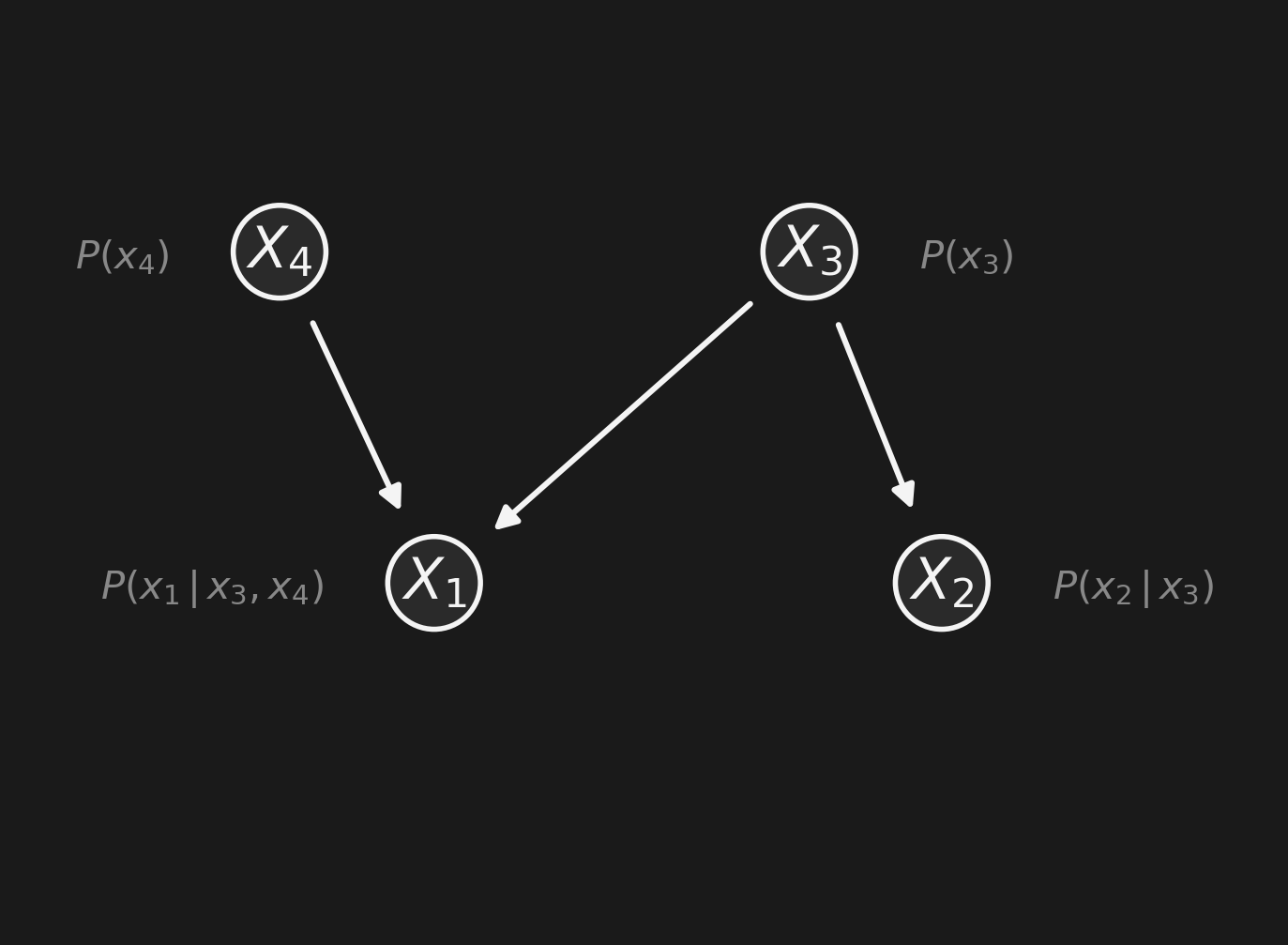
For 4 binary variables, the full joint needs \(2^4 - 1 = 15\) numbers. This Bayes net needs how many?

2値変数4つの場合、完全な同時分布 には \(2^4 - 1 = 15\) 個の数が必要。 このベイズネットは何個で済むか？

~45 sec. Pose the question. Don’t reveal yet. Per-node counts hidden — let students count for themselves. Hint verbally: “each node contributes 2^(#parents) numbers.” Then advance to the reveal.

How compact is this? — answerどれくらいコンパクトか？ — 答え

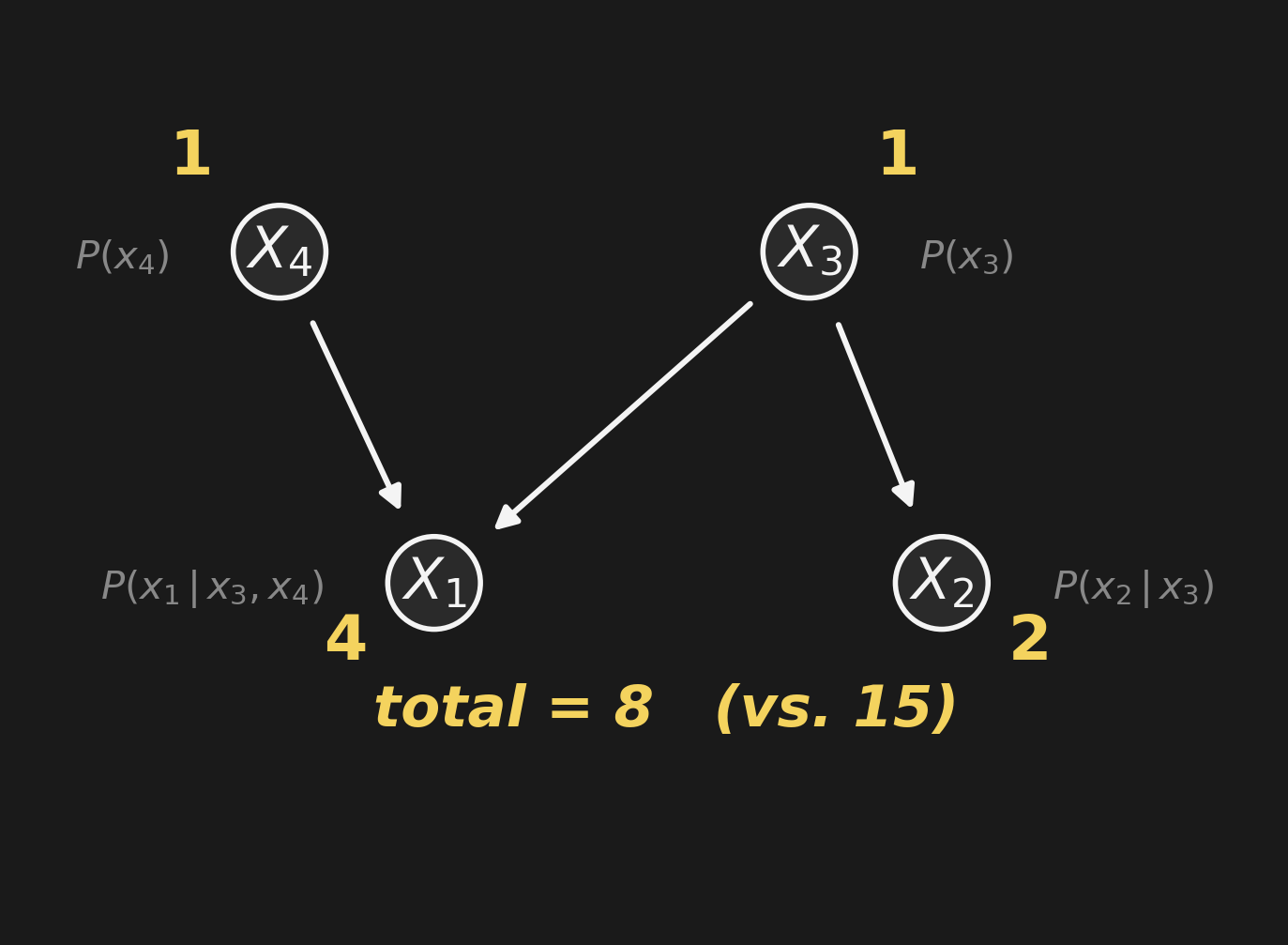
8 vs. 15. Modest gain here — exponential gain at scale.

8 個 vs. 15 個。ここでは控えめな差 — 規模が大きくなると指数的な差に。

~45 sec. The Pearl psychic-friend example. Per-node counts revealed on the figure. The “vs 15” is the punchline. Mention this gets more dramatic fast: 10 binary vars → 1023 vs maybe 30. 50 binary vars → 10^15 vs maybe a few hundred.

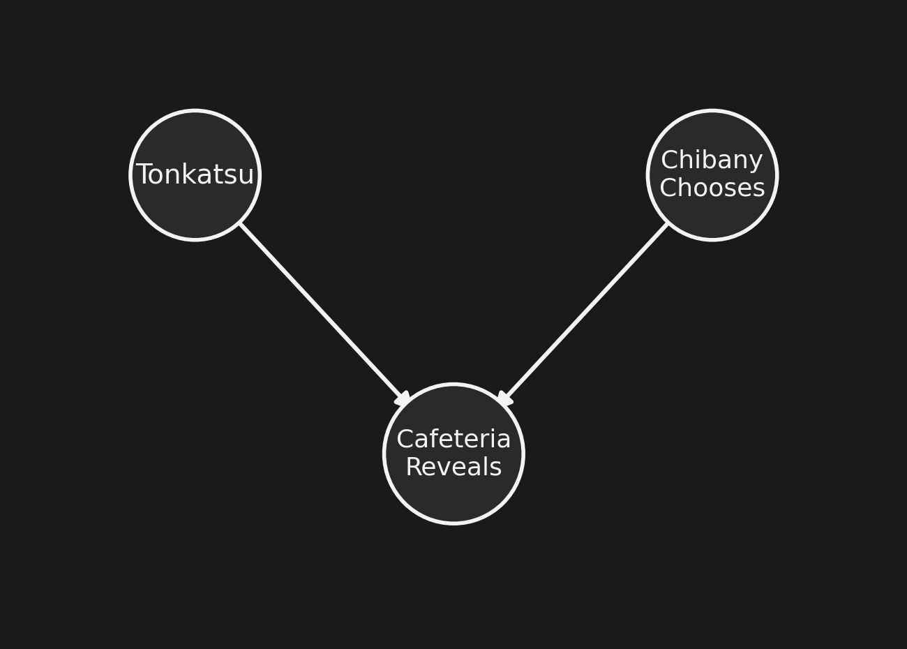
Same network, different costume同じネット、違う衣装

Chibany versionチバニー版

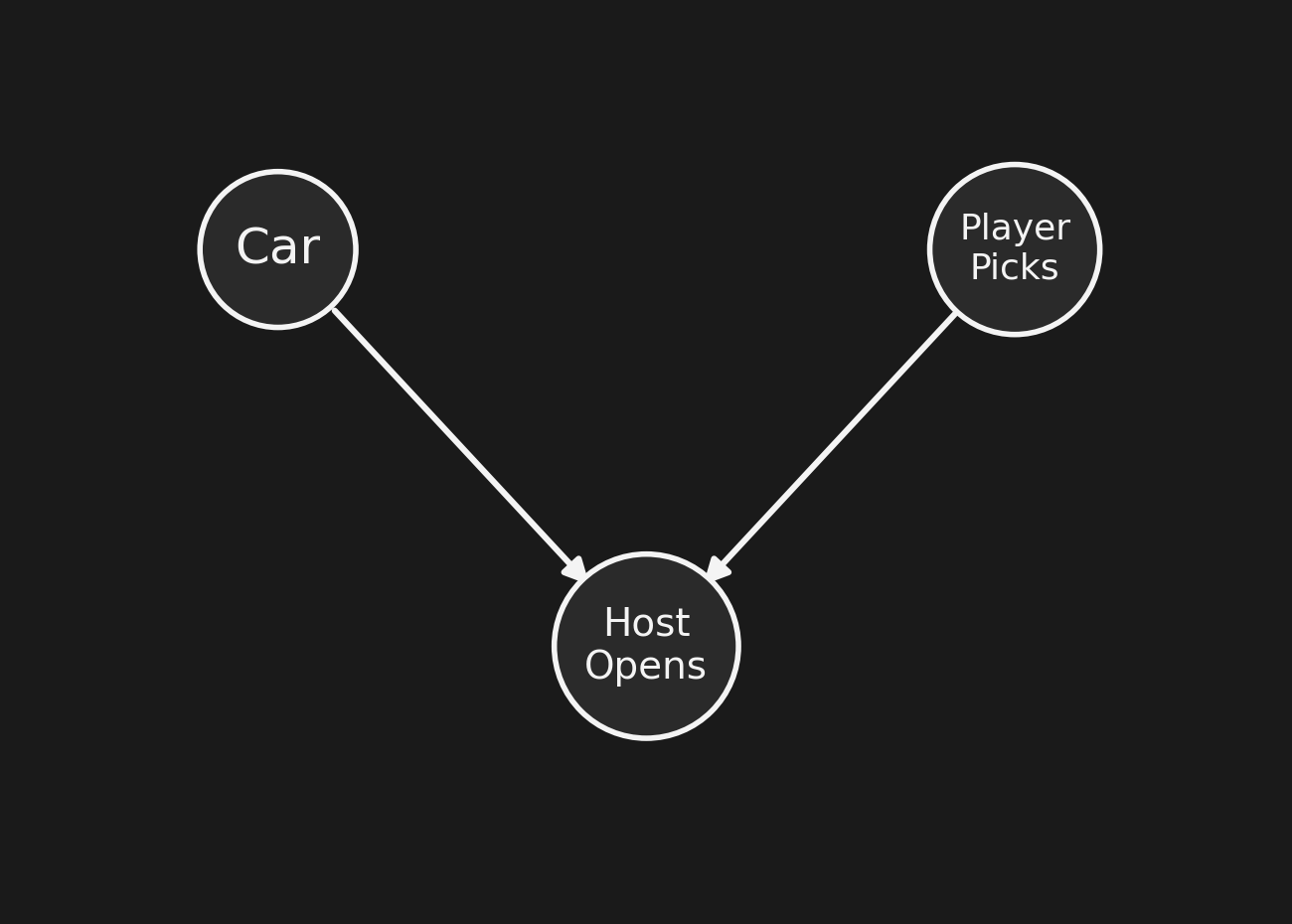
Classic Monty Hall古典的なモンティ・ホール

Car / Host / Player and Tonkatsu / Cafeteria / Chibany — literally the same network. The 2/3 vs 1/3 answer is structural.

車 / ホスト / プレイヤー と トンカツ / 店員 / チバニー — 文字通り 同じネットワーク。 2/3 vs 1/3 の答えはネットワーク構造から来る。

~45 sec. Bridge from Chibany to the cultural reference. Some students will have heard of Monty Hall before; now they know what makes it work structurally.

Poll — Bayes-net factorizationポール — ベイズネット因数分解

In the Chibany Monty Hall network (Tonkatsu → Reveals ← Chooses), the joint \(P(T, R, C)\) factorizes as:

チバニーのモンティ・ホールネット（トンカツ → 公開 ← 選択）において、 同時分布 \(P(T, R, C)\) の因数分解は：

• A. \(P(T) \, P(C) \, P(R \mid T, C)\)
• B. \(P(T \mid C) \, P(C) \, P(R)\)
• C. \(P(T) \, P(C \mid T) \, P(R \mid C)\)
• D. Cannot factorize — all three are dependent.

• A. \(P(T) \, P(C) \, P(R \mid T, C)\)
• B. \(P(T \mid C) \, P(C) \, P(R)\)
• C. \(P(T) \, P(C \mid T) \, P(R \mid C)\)
• D. 因数分解できない — 3つすべて従属。

~60 sec. Commit-before-reveal. Each node, given its parents, contributes one factor. T and C have no parents → marginals. R has T and C as parents → conditional on both. (A) is correct.

Poll — answerポール — 答え

A. \(P(T) \, P(C) \, P(R \mid T, C)\)A. \(P(T) \, P(C) \, P(R \mid T, C)\)

Each node, given its parents, contributes one factor. \(T\) and \(C\) are root nodes (no parents) → marginals. \(R\) is a child of both → conditional on both.

各ノードは、その親ノードに条件付けられた因子を1つ提供する。 \(T\) と \(C\) は根ノード（親なし）→ 周辺確率。 \(R\) は両方の子 → 両方に条件付けられた条件付き確率。

~45 sec. (B) gets the conditioning backwards. (C) inserts a non-existent edge C→T. (D) confuses dependence with non-factorization — a Bayes net can have dependent variables AND still factorize.

d-separation + Bayes-Balld分離 + ベイズボール

Reading independence off the graphグラフから独立性を読み取る

The Markov factorization tells us how the joint factors. But what about conditional independence?

Three patterns to know — every Bayes net is built from these:

• Chain: \(A \to B \to C\)
• Fork: \(A \leftarrow B \to C\)
• Collider: \(A \to B \leftarrow C\)

Conditioning on \(B\) behaves differently in each.

マルコフ因数分解は、同時分布の 因数分解 を教えてくれます。 では 条件付き独立性 はどうでしょうか？

3つのパターン — どのベイズネットもこれらから組み立てられている：

• チェーン（鎖）: \(A \to B \to C\)
• フォーク（分岐）: \(A \leftarrow B \to C\)
• コライダー（合流）: \(A \to B \leftarrow C\)

\(B\) に条件付けるとき、それぞれ 違う 振る舞いをします。

~60 sec. Set up the 3-slide build-up. Tell them ahead of time: collider is the weird one. The setup primes them to look for the asymmetry.

Chain: A → B → Cチェーン: A → B → C

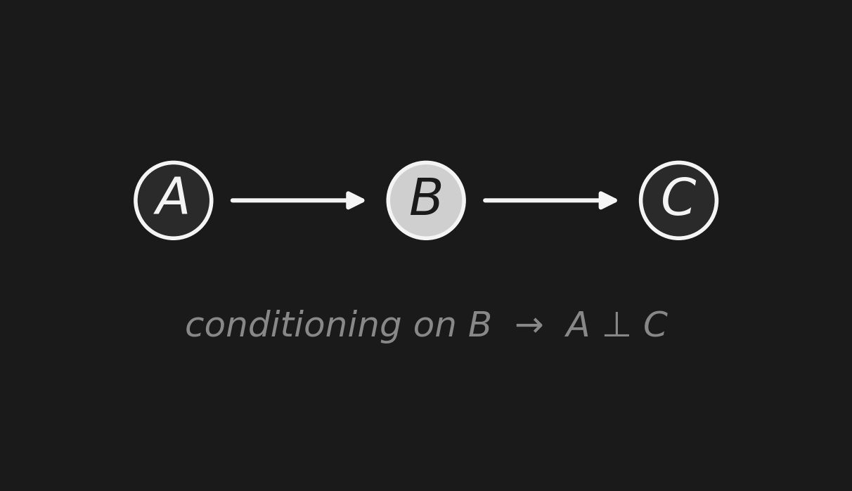
Conditioning on the middle node blocks information flow.

\[A \;\perp\; C \;\mid\; B\]

中間ノードに条件付けると、情報の流れは 遮断 される。

\[A \;\perp\; C \;\mid\; B\]

~60 sec. Example: Sleep → Caffeine → Alertness. Knowing caffeine intake makes sleep and alertness conditionally independent — caffeine “absorbs” all the sleep-info relevant to alertness.

Fork: A ← B → Cフォーク: A ← B → C

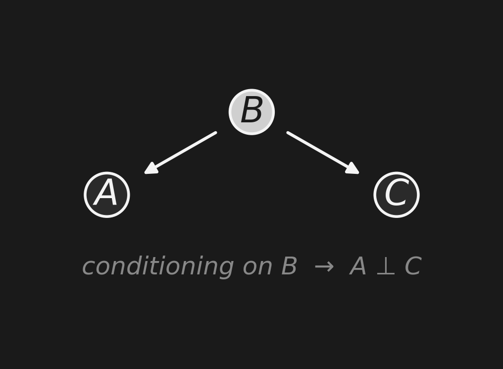
A common cause. Conditioning on the cause blocks information flow.

\[A \;\perp\; C \;\mid\; B\]

共通原因。原因に条件付けると、情報の流れは 遮断 される。

\[A \;\perp\; C \;\mid\; B\]

~60 sec. Example: a common-cause structure — Genetics → both Height and Vocabulary. Knowing genetics makes the two seemingly correlated outcomes conditionally independent.

Collider: A → B ← Cコライダー: A → B ← C

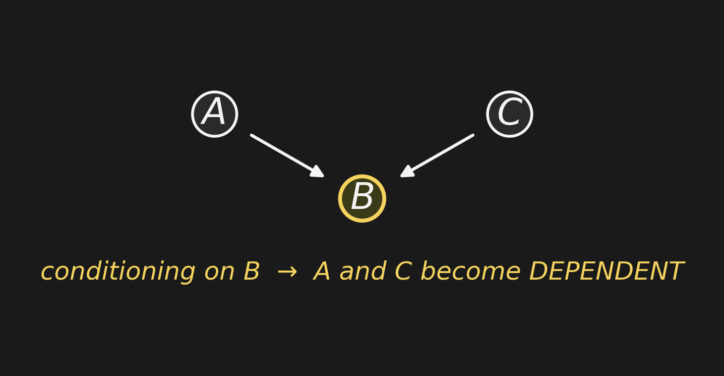
A common effect. Conditioning on the effect induces dependence between the otherwise-independent causes.

\[A \;\perp\; C \quad\text{but}\quad A \;\not\perp\; C \;\mid\; B\]

This is backwards from chain and fork. It’s the surprise of the lecture.

共通の結果。結果に条件付けると、もともと独立だった原因間に依存性が 生じる。

\[A \;\perp\; C \quad\text{しかし}\quad A \;\not\perp\; C \;\mid\; B\]

これはチェーンやフォークと 逆向き。今日の講義の意外なポイント。

~75 sec. THE key concept for the rest of the lecture. Flag it explicitly: this looks wrong, and yet it’s right. We’ll see WHY in Block 5 (explaining away). For now, just absorb the rule: collider conditioning OPENS the path.

Markov blanketマルコフブランケット

Definition. The Markov blanket of node \(X\):

• parents of \(X\)
• children of \(X\)
• other parents of \(X\)’s children (the “spouses”)

Conditioning on the Markov blanket makes \(X\) independent of everything else in the network.

The spouses are the non-obvious part — they’re there because of collider conditioning flowing through \(X\)’s children.

定義. ノード \(X\) のマルコフブランケット：

• \(X\) の 親
• \(X\) の 子
• \(X\) の子の 他の親（「配偶者」）

マルコフブランケットに条件付けると、\(X\) はネットワーク中の 他のすべてから独立 になる。

配偶者は自明でないところ — \(X\) の子を通って流れる コライダーへの条件付け のために含まれる。

~90 sec. The spouses bit is the non-obvious part — that’s collider-conditioning flowing through children’s other parents. Use the figure to point.

Bayes-Ball: interactive demoベイズボール：インタラクティブデモ

The widget runs 3 scripted scenarios: 1. Chain with B conditioned — ball blocks at B. 2. Collider with B not conditioned — ball blocks at B. 3. Collider with B conditioned — ball passes through to C.

Keyboard: 1/2/3 to pick scenario; space or arrow-right to step; r to reset. Each scenario takes ~90 sec to run through. Don’t open-ended-explore. ~5 min total for the widget.

Poll — collider conditioningポール — コライダーの条件付け

You see the cafeteria worker reveal a bento (not Chibany’s pick, not tonkatsu). You haven’t been told which bento Chibany picked. Does the worker’s choice tell you anything about Chibany’s pick?

店員がお弁当を1つ公開する（チバニーの選択でもなく、トンカツでもない）。 チバニーがどれを選んだかはまだ知らない。店員の選択は、チバニーの選択について 何か教えてくれるだろうか？

• A. Yes — the worker’s choice and Chibany’s pick become dependent.
• B. No — they were independent before, so they’re still independent.
• C. Only if you also know which bento has the tonkatsu.
• D. Chibany’s pick was random, so nothing tells you about it.

• A. はい — 店員の選択とチバニーの選択は従属になる。
• B. いいえ — もともと独立だったので、今も独立。
• C. トンカツの位置も知っている場合のみ。
• D. チバニーの選択はランダムなので、何も教えてくれない。

~60 sec. (B) is the natural mistake — that’s exactly the misconception we need to dislodge. Watch for students who pick it; they need to see Block 5 (explaining away) for the resolution.

Poll — answerポール — 答え

A. Yes — collider conditioning induces dependence.A. はい — コライダーの条件付けは依存性を生み出す。

The worker’s choice constrains Chibany’s pick: if the worker opened box 3, Chibany must have picked box 1 or 2 (otherwise the worker would have opened something else). The choices are now correlated through the constraint.

This is explaining away — Block 5.

店員の選択はチバニーの選択を制約する：店員が3番を開けたなら、 チバニーは1番か2番を選んだに違いない（さもなければ店員は別の箱を開けたはず）。 2つの選択は制約 を通じて 相関する。

これが 説明はがし — ブロック5。

~60 sec. Pay off the surprise. The reasoning is “given what we observed, what ASSIGNMENTS to the parents are consistent?” — and that’s a constraint on the joint over parents, which means they’re now dependent.

Explaining away説明はがし

Sprinkler / Rain / Wet grassスプリンクラー / 雨 / 濡れた芝生

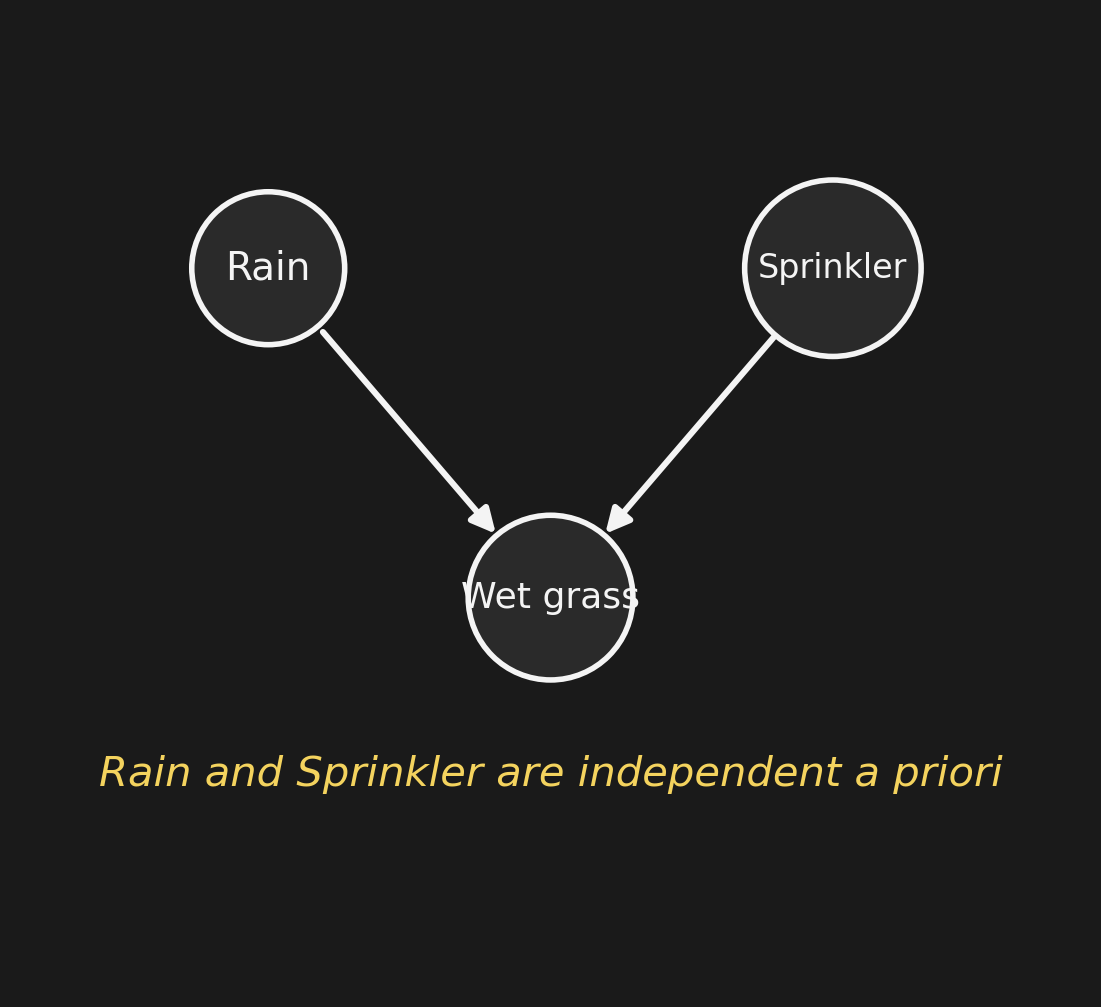
Three nodes: Rain (\(R\)), Sprinkler (\(S\)), Wet grass (\(W\)). Two independent causes of wet grass. A priori, \[P(R) = 0.3, \quad P(S) = 0.3, \quad P(R, S) = P(R)\,P(S).\] Rain and Sprinkler are independent. The grass is wet if either cause fires: \[W = 1 \iff (R = 1)\ \text{or}\ (S = 1). \quad\text{(deterministic OR)}\]

\(R\), \(S\), \(W\) from here on.

3つのノード：雨 (\(R\))、スプリンクラー (\(S\))、濡れた芝生 (\(W\))。濡れた芝生の独立な2つの原因。事前分布は、 \[P(R) = 0.3, \quad P(S) = 0.3, \quad P(R, S) = P(R)\,P(S).\] 雨とスプリンクラーは 独立。どちらか の原因が起これば芝生は濡れる： \[W = 1 \iff (R = 1)\ \text{または}\ (S = 1). \quad\text{(決定的 OR)}\]

以降、\(R\), \(S\), \(W\) と略記。

~60 sec. Establish the baseline: nothing observed, both causes are independent of each other. Standard collider setup.

Observe wet grass濡れた芝生を観測

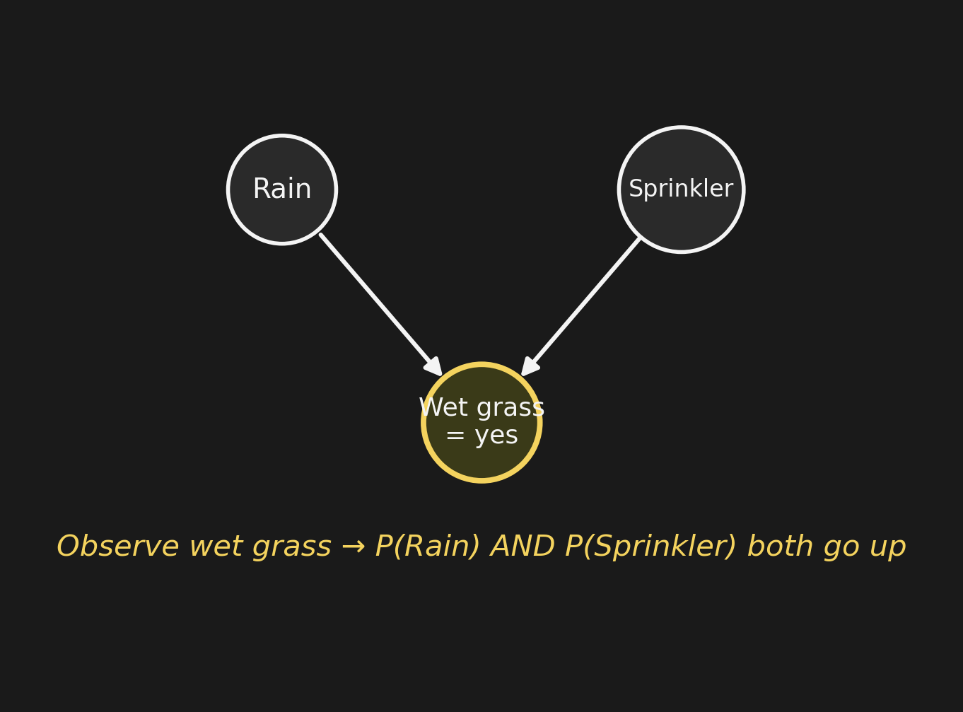
Now we walk outside: the grass is wet (\(W = 1\)). Both probabilities rise: \[P(R \mid W) \approx 0.59, \quad P(S \mid W) \approx 0.59.\] Either cause is now more plausible — the observation supports both.

さて、外に出ると：芝生が濡れている (\(W = 1\))。両方の確率が 上がる： \[P(R \mid W) \approx 0.59, \quad P(S \mid W) \approx 0.59.\] どちらの原因も今や確からしくなる — 観測は両方を支持する。

~75 sec. The “competition” hasn’t happened yet — the wetness elevates both hypotheses. Under the deterministic OR these are exact: P(R|W) = P(S|W) = 10/17 ≈ 0.59 (0.3 → 0.59, roughly doubled).

Also learn sprinkler was onさらに、スプリンクラーが作動していたと知る

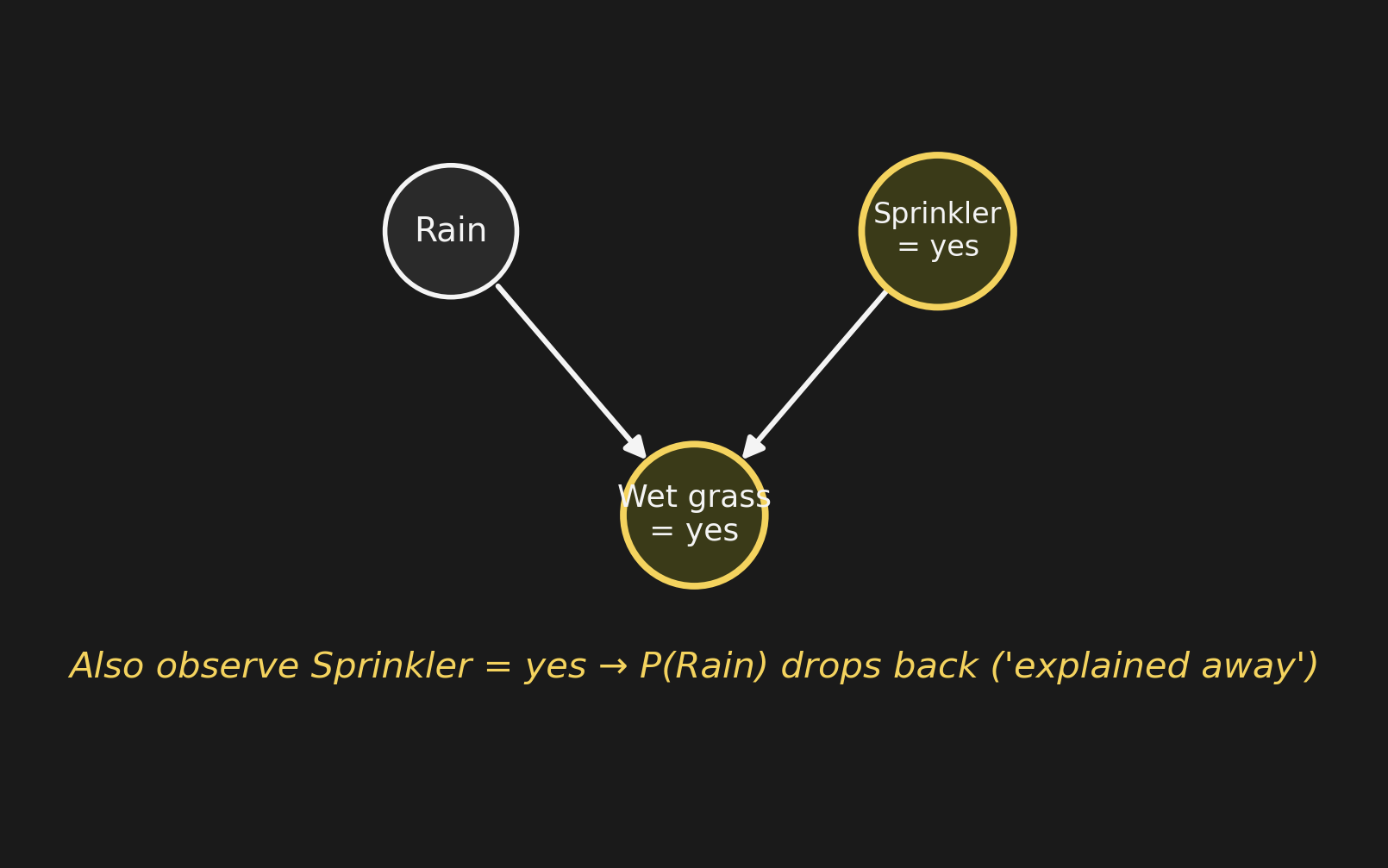
A neighbor mentions: “I saw your sprinkler running this morning.” So \(S = 1\). Now: \[P(R \mid W, S = 1) = 0.3 = P(R).\] Rain’s probability drops all the way back to its prior — sprinkler already “explains” the wetness, so wet grass tells us nothing more about rain.

Conditioning on the collider’s parents and the collider itself induces this competition. That’s explaining away.

近所の人が言う：「今朝あなたのスプリンクラーが動いているのを見たよ。」つまり \(S = 1\)。今度は： \[P(R \mid W, S = 1) = 0.3 = P(R).\] 雨の確率が 事前分布まで完全に戻る — スプリンクラーが濡れていることを既に「説明」したので、 濡れた芝生は雨について もう何も教えてくれない。

コライダーの親 と コライダー自身に条件付けることで、この競合が生まれる。 これが説明はがし。

~90 sec. THE key numerical reveal. Rain went 0.3 → 0.59 → 0.30 — it rises on wet grass, then returns EXACTLY to its prior once the sprinkler is known on. With a deterministic OR, S=1 makes wet grass certain regardless of rain, so W carries zero further information about R: P(R|W,S=1) = P(R) = 0.3 exactly. The sprinkler fully “explains” the wetness. (A noisy OR would leave R slightly above prior — the residual is the signature of non-determinism; we keep the clean deterministic version here.) Aside worth saying aloud: if instead the grass were wet with S=0, only rain is left to explain it, so P(R|W,S=0)=1.

What just happened今、何が起きたのか

The numbers:

Conditioning set	\(P(R = 1)\)
nothing	0.30
\(W = 1\)	0.59
\(W = 1,\, S = 1\)	0.30

Rain rose, then fell back to its prior. The fall is explaining away.

数値の変化：

条件付け	\(P(R = 1)\)
なし	0.30
\(W = 1\)	0.59
\(W = 1,\, S = 1\)	0.30

雨の確率は上がり、事前分布まで戻った。下がる部分が 説明はがし。

The take-home in one sentence:

Conditioning on a common effect (the collider) makes the independent causes dependent. Then learning one cause reduces the support for the other.

Same mechanism, two stages.

一文でまとめると：

共通の結果（コライダー）に条件付けると、独立だった原因が 従属になる。 そして一つの原因を学ぶと、もう一つの原因への支持が 減る。

同じメカニズム、2つの段階。

~75 sec. The two-column summary. Numbers on the left, take-home on the right. The “two stages” framing is important: stage 1 = conditioning on the collider induces dependence; stage 2 = the dependence is a competition for explaining the observation.

Why Chibany should switch — explainedチバニーが箱を変えるべき理由 — 説明はがしで

Remember Monty Hall? Tonkatsu and Chibany’s pick were independent a priori. We then conditioned on the collider (the worker’s reveal).

That’s explaining away.

The worker had to open some box. If Chibany picked correctly (T = 1), the worker had a free choice. If Chibany picked wrong (T ≠ 1), the worker was forced to open the specific other box. The “forcing” is what makes the posterior favor switching.

モンティ・ホールを覚えていますか？トンカツとチバニーの選択は、事前には独立でした。 そして コライダー（店員の公開）に条件付けた。

それが説明はがし。

店員は どれか 箱を開けないといけない。もしチバニーが正解を選んでいたら（T = 1）、 店員には自由な選択肢があった。もし間違っていたら（T ≠ 1）、店員は特定の箱を 開けるしか なかった。この「強制」が、事後分布を「変える」方に傾けるのです。

~90 sec. Tie the threads: Monty Hall WAS explaining away, all along. The worker’s reveal is the collider; conditioning on it makes Chibany’s pick and tonkatsu location dependent — which is what gives us the 2/3 answer.

Break休憩

10-min break. The cat is Callie on her chair. Stretch, hydrate. We’re at 1:12, returning at 1:22 for the causal half.

Observation → intervention観測 → 介入

A claim from the dentist歯医者からの主張

Chibany is at the dentist. “People with yellow teeth,” the dentist says, “tend to have higher rates of lung cancer.”

Chibany asks: “Should I whiten my teeth?”

チバニーは歯医者で。「歯が黄色い人は」と歯医者が言う、「肺がんの率が高い傾向がある。」

チバニーが聞く：「歯を白くしたほうがいい？」

~45 sec. Set up the joke; the answer is obviously no. The interesting question is WHY no. The DAG language we just developed gives us the precise answer.

The confound共通原因（交絡）

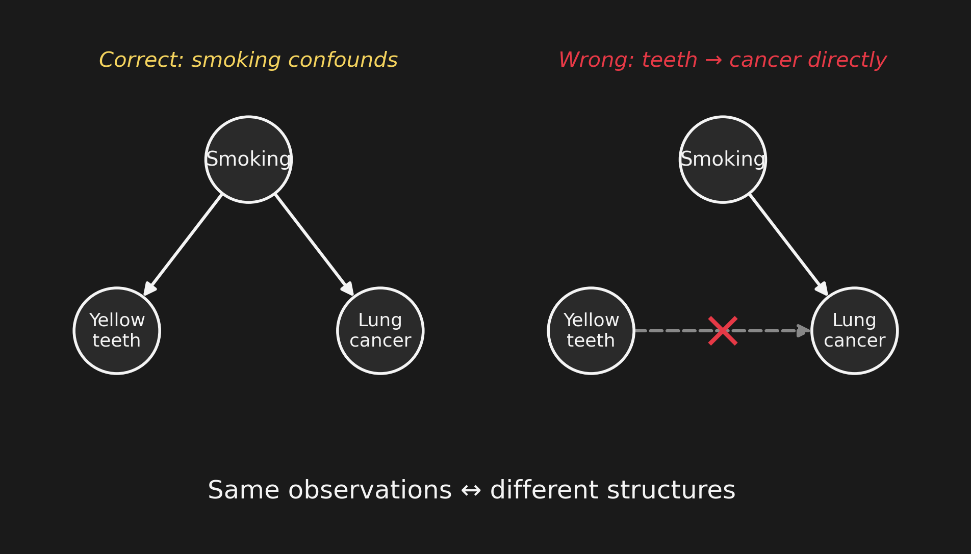
Three variables: Smoking (\(S\)), Yellow teeth (\(T\)), Lung cancer (\(L\)). Two structures give exactly the same statistical correlation:

• \(S\) causes both \(T\) and \(L\) (correct).
• \(T\) directly causes \(L\) (wrong, but observationally indistinguishable).

Observation alone cannot tell them apart. You’d see the same correlation either way.

\(S\), \(T\), \(L\) from here on.

3つの変数：喫煙 (\(S\))、黄色い歯 (\(T\))、肺がん (\(L\))。2つの構造が まったく同じ 統計的相関を生む：

• \(S\) が \(T\) と \(L\) の両方の原因（正しい）。
• \(T\) が直接 \(L\) を引き起こす（誤りだが、観測上は区別できない）。

観測だけではこの2つを区別できません。 どちらの構造でも同じ相関が見られる。

以降、\(S\), \(T\), \(L\) と略記。

~90 sec. The point: correlation under-determines causal structure. To distinguish, you need something more — and that’s what intervention gives you.

Three causal stories, one correlation: chain1つの相関、3つの因果ストーリー：チェーン

Story 1 (chain): \(T \to S \to L\) — yellow teeth cause smoking, smoking causes lung cancer. Implausible, but observationally consistent.

Conditional independence: \(T \perp L \mid S\).

ストーリー1（チェーン）: \(T \to S \to L\) — 黄色い歯が喫煙の原因で、 喫煙が肺がんの原因。実際にはありそうにないが、観測上は整合的。

条件付き独立性: \(T \perp L \mid S\)。

~45 sec. Walk through the first story. Each story is observationally consistent with the same correlation between T and L — that’s the point.

Three causal stories, one correlation: fork1つの相関、3つの因果ストーリー：フォーク

Story 2 (fork): \(T \leftarrow S \to L\) — smoking causes both. The real story for the smoking-yellow-teeth-cancer triangle.

Conditional independence: \(T \perp L \mid S\).

Identical to chain! Observation cannot tell these apart.

ストーリー2（フォーク）: \(T \leftarrow S \to L\) — 喫煙が両方の原因。 喫煙-黄色い歯-肺がんの三角関係の 本当の ストーリー。

条件付き独立性: \(T \perp L \mid S\)。

チェーンと同一！ 観測ではこの2つを区別できません。

~45 sec. THE key reveal: chain and fork are observationally identical. Same conditional-independence pattern. Same joint distribution. The arrows point different ways but observation can’t see arrowheads.

Three causal stories, one correlation: collider1つの相関、3つの因果ストーリー：コライダー

Story 3 (collider): \(T \to S \leftarrow L\) — yellow teeth and lung cancer each independently cause smoking (also implausible, but bear with it).

Conditional dependence: \(T \not\perp L \mid S\).

Observationally distinct — but the wrong structure for a smoking confound. Most real-world confounds are forks, indistinguishable from chains.

ストーリー3（コライダー）: \(T \to S \leftarrow L\) — 黄色い歯と肺がんが それぞれ独立に喫煙の原因（これもありそうにないが、お付き合いください）。

条件付き従属性: \(T \not\perp L \mid S\)。

観測で区別できる — しかし、喫煙の交絡には合わない構造。 現実の交絡の多くはフォークで、チェーンとは区別できません。

~45 sec. Collider is observationally distinct from chain/fork — but it’s not the structure we worry about for confounding. The under-determination of chain-vs-fork is the actual problem.

What we need必要なもの

What observation tells you:

• statistical dependence
• joint distribution
• can’t disambiguate chain from fork

This is Level 1 of Pearl’s ladder.

観測が教えてくれること：

• 統計的従属性
• 同時分布
• チェーンとフォークの区別はつかない

これがパールの梯子の レベル1。

What intervention would do:

• cut incoming arrows
• reveal the cause
• break Markov equivalence

This is Level 2 — coming up next.

介入なら何ができるか：

• 入ってくる矢印を切る
• 原因を明らかにする
• マルコフ同値を破る

これが レベル2 — 次に登場。

~60 sec. Set up Block 7. Pearl’s ladder: Level 1 = seeing, Level 2 = doing, Level 3 = counterfactuals. We’ll stay on 1 and 2.

The do-operatordo演算子

The original network元のネットワーク

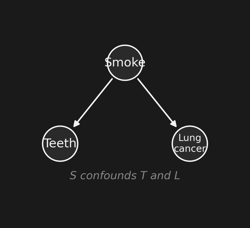
\(S \to T\) (smoking causes yellow teeth), \(S \to L\) (smoking causes lung cancer). \(T\) and \(L\) are correlated because of the common cause \(S\).

If we observe \(T = \text{yellow}\), we update our belief about \(S\), and therefore about \(L\). Hence \(P(L \mid T = \text{yellow}) > P(L)\).

\(S \to T\)（喫煙が歯を黄色くする）、\(S \to L\)（喫煙が肺がんの原因）。 \(T\) と \(L\) は共通原因 \(S\) を通じて 相関する。

\(T = \text{黄色}\) を 観測 すると、\(S\) についての信念が更新され、 そのため \(L\) についても更新される。だから \(P(L \mid T = \text{黄色}) > P(L)\)。

~60 sec. Establish the observational baseline: P(L|T) > P(L). That’s the “yellow teeth correlate with cancer” claim from the dentist.

do(T = white): cut the incoming arrowdo(T = 白): 入ってくる矢印を切る

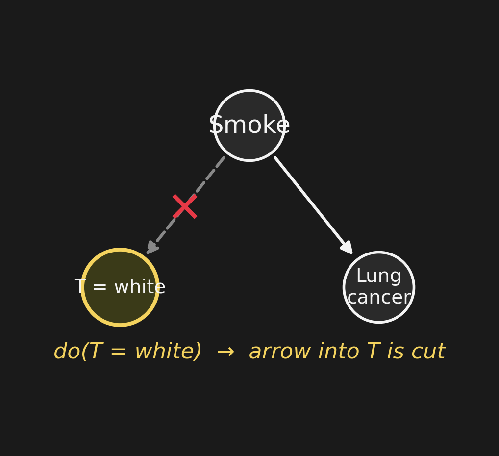
Graph surgery. We set \(T = \text{white}\) by intervention — we paid for whitening. The intervention cuts the incoming arrow \(S \to T\).

Why cut? Because \(T\) is no longer being generated by smoking. \(T\) is being generated by Chibany’s wallet. The mechanism changed.

グラフ手術. 介入によって \(T = \text{白}\) にする — 歯を白くする処置にお金を払った。 介入は 入ってくる矢印 \(S \to T\) を切断する。

なぜ切る？\(T\) はもはや喫煙によって 生成されていない から。\(T\) はチバニーの財布に よって生成されている。メカニズムが変わったのです。

~90 sec. THE key conceptual move. Spend time on this: “the mechanism that generates T has changed.” Pearl’s phrasing: do() replaces the conditional probability table for T with a fixed value.

Compute P(L | do(T = white))P(L | do(T = 白)) を計算

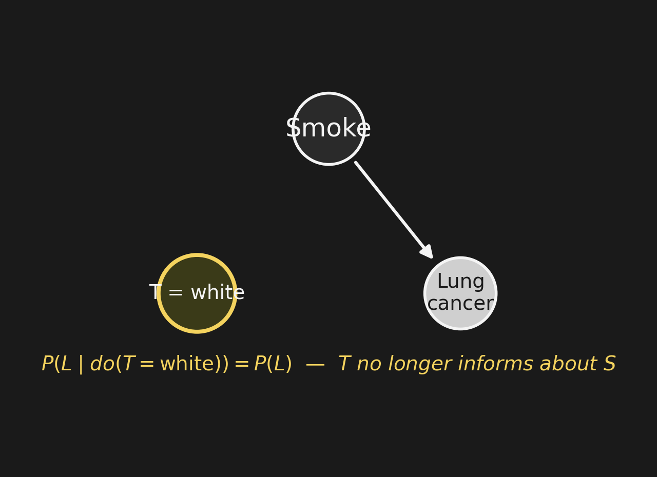
After surgery, \(T\) has no parents. The factorization becomes: \[P(S, L, T = \text{white}) = P(S) \, P(L \mid S).\]

Marginalize over \(S\) to get \(P(L \mid do(T = \text{white}))\): \[P(L \mid do(T = \text{white})) = \sum_S P(L \mid S) \, P(S) = P(L).\]

Intervention severed the path from \(T\) back to \(L\) through \(S\). \(T\) no longer carries any information about \(S\), so knowing \(T\) tells you nothing new about \(L\).

手術後、\(T\) には親がない。因数分解は次のようになる： \[P(S, L, T = \text{白}) = P(S) \, P(L \mid S).\]

\(S\) について周辺化して \(P(L \mid do(T = \text{白}))\) を得る： \[P(L \mid do(T = \text{白})) = \sum_S P(L \mid S) \, P(S) = P(L).\]

介入は \(T\) から \(S\) を経由して \(L\) へ戻る経路を断ち切った。 \(T\) はもう \(S\) について何の情報も運ばないので、\(T\) を知っても \(L\) について新しいことは何も分からない。

~2 min. Show the marginalization step explicitly. The intuition: in the observational world, T was a SIGNAL of S; in the intervened world, T is just a value we set, with no relation to S.

\(P(L \mid T)\) vs. \(P(L \mid do(T))\)\(P(L \mid T)\) vs. \(P(L \mid do(T))\)

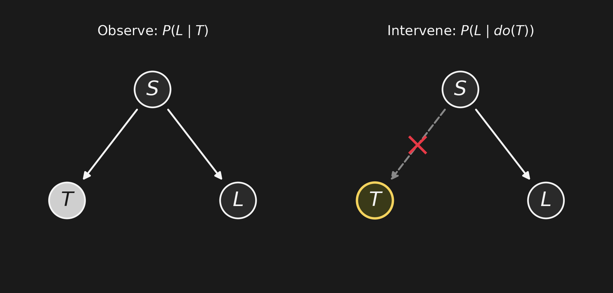
Same notation, different operation, different answer.

• \(P(L \mid T)\): passive observation. Yellow teeth tell you about smoking.
• \(P(L \mid do(T))\): active intervention. Yellow teeth tell you about the dentist’s bill.

同じ記号、違う操作、違う答え。

• \(P(L \mid T)\): 受動的な観測。黄色い歯は喫煙について教えてくれる。
• \(P(L \mid do(T))\): 能動的な介入。黄色い歯は歯科医の請求書について教えてくれる。

~60 sec. The two-column side-by-side. Drive home: the SAME mathematical syntax (P(L | something)) means TWO DIFFERENT THINGS depending on whether the “something” is observed or intervened.

Poll — do vs. conditionポール — do vs. 条件付け

In the smoking network \(S \to T, S \to L\), Chibany pays to whiten their teeth (intervention: \(T = \text{white}\)).

What is \(P(\text{lung cancer} \mid do(T = \text{white}))\)?

喫煙ネットワーク \(S \to T, S \to L\) で、チバニーがお金を払って歯を白くする （介入：\(T = \text{白}\)）。

\(P(\text{肺がん} \mid do(T = \text{白}))\) は？

• A. Lower than \(P(\text{lung cancer})\) — white teeth predict less smoking.
• B. Same as \(P(\text{lung cancer})\) — intervention cuts the \(S \to T\) edge.
• C. Higher than \(P(\text{lung cancer})\) — paint chemicals are toxic.
• D. Unknown without more data.

• A. \(P(\text{肺がん})\) より低い — 白い歯は喫煙の少なさを予測する。
• B. \(P(\text{肺がん})\) と同じ — 介入は \(S \to T\) の辺を切る。
• C. \(P(\text{肺がん})\) より高い — 塗料の化学物質は有毒。
• D. データが足りない。

~75 sec. (A) is the seductive observational answer. (B) is correct: the intervention severed the back-door path from T to L through S.

Poll — answerポール — 答え

B. Same as \(P(\text{lung cancer})\).B. \(P(\text{肺がん})\) と同じ。

The intervention cuts the \(S \to T\) edge. \(T\) no longer informs about \(S\), and the path from \(T\) to \(L\) (which went through \(S\)) is severed.

(A) is the trap — it’s the right answer if you observe \(T\), but the wrong answer if you intervene on \(T\).

介入は \(S \to T\) の辺を切る。\(T\) はもう \(S\) について何も教えてくれず、 \(T\) から（\(S\) を経由して）\(L\) への経路は断ち切られた。

(A) は罠 — \(T\) を 観測 するなら正しい答え、\(T\) に 介入 するなら間違った答え。

~60 sec. Watch the room. If more than half pick (A), spend an extra 30 sec on why — the temptation is the entire reason this poll exists.

Causal cognition — the blicket detector因果認知 — ブリケット検出器

The blicket detectorブリケット検出器

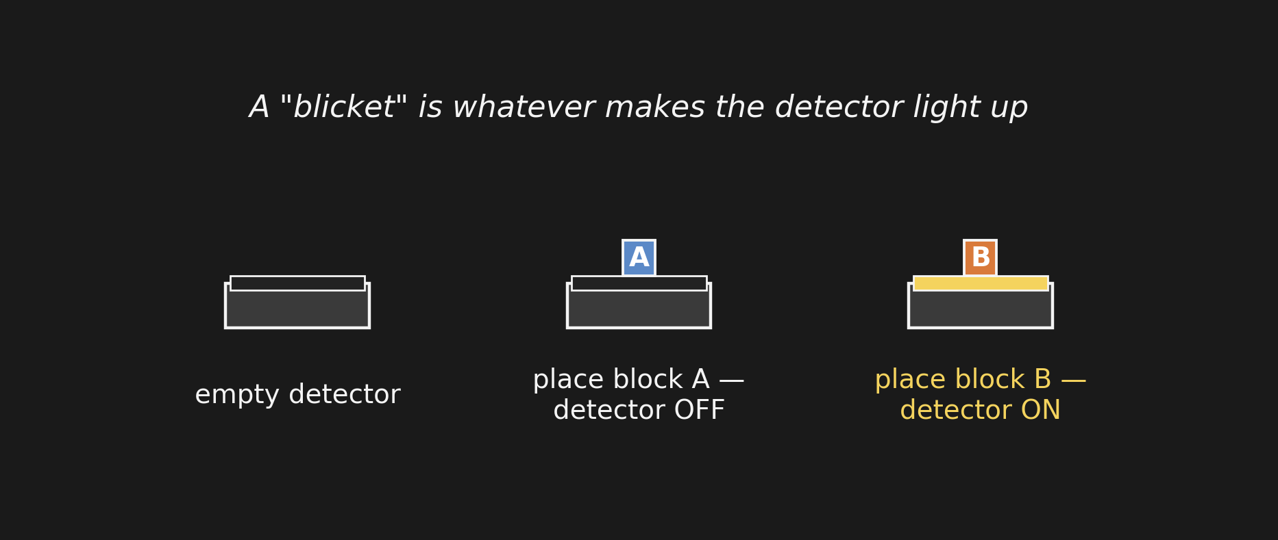
A children’s experiment (Gopnik & Sobel, 2000). A “blicket” is whatever makes the machine light up. Children watch blocks placed on the detector and infer which blocks are blickets.

子ども向けの実験（ゴプニックとソベル、2000）。「ブリケット」とは、機械を光らせる ものすべて。子どもは積み木が検出器に置かれるのを見て、どの積み木がブリケットかを推論する。

~60 sec. Set up the experiment. The key: kids are doing causal inference, not just statistical inference. They need to disentangle which block is doing the work.

The experiment as a Bayes netベイズネットとしての実験

The physical setup:

• A machine (“detector”) that lights up.
• A collection of blocks. Each block is or isn’t a blicket.
• Place blocks on the machine; observe whether it lights up.

The child’s job: figure out which blocks are blickets.

物理的な構造：

• 光る機械（「検出器」）。
• いくつかの積み木。各積み木はブリケットかそうでないか。
• 積み木を機械に置く；光るかどうかを観測。

子どもの仕事：どの積み木がブリケットかを見つけ出す。

The Bayes net:

For two blocks \(A\), \(B\):

• \(A\)-blicket? → Detector lights
• \(B\)-blicket? → Detector lights

A collider: detector is the common effect.

Each trial conditions on the collider. Inference is explaining away.

ベイズネット：

積み木 \(A\)、\(B\) について：

• \(A\) はブリケット？ → 検出器が光る
• \(B\) はブリケット？ → 検出器が光る

コライダー：検出器が共通の結果。

各試行は コライダーへの条件付け。 推論は 説明はがし。

~90 sec. The two-column bridge: experiment on the left, Bayes net on the right. Show the audience that they already have the formal tools to predict what happens — it’s a collider, two trials = two observations of the collider, explaining away is the inference.

Backwards blockingバックワード・ブロッキング

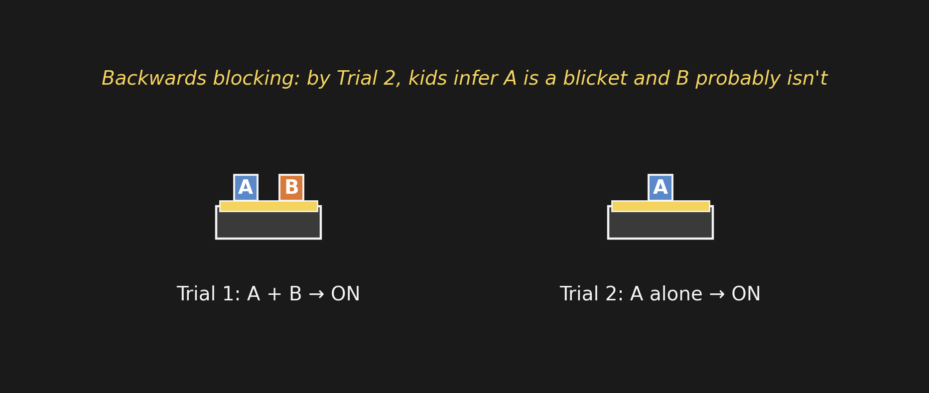
• Trial 1: A and B together → detector ON.
• Trial 2: A alone → detector ON.

After Trial 2, what do kids think about B?

• 試行1: AとBを一緒に → 検出器 ON。
• 試行2: Aだけ → 検出器 ON。

試行2の後、子どもはBについてどう思う？

~60 sec. Pose the inference. A is clearly a blicket — alone, it turns on the detector. What about B? After Trial 1 alone, B could go either way. After Trial 2, A “explains” the Trial 1 result, and B’s blicket-status drops.

Children match the Bayes net子どもはベイズネットと一致する

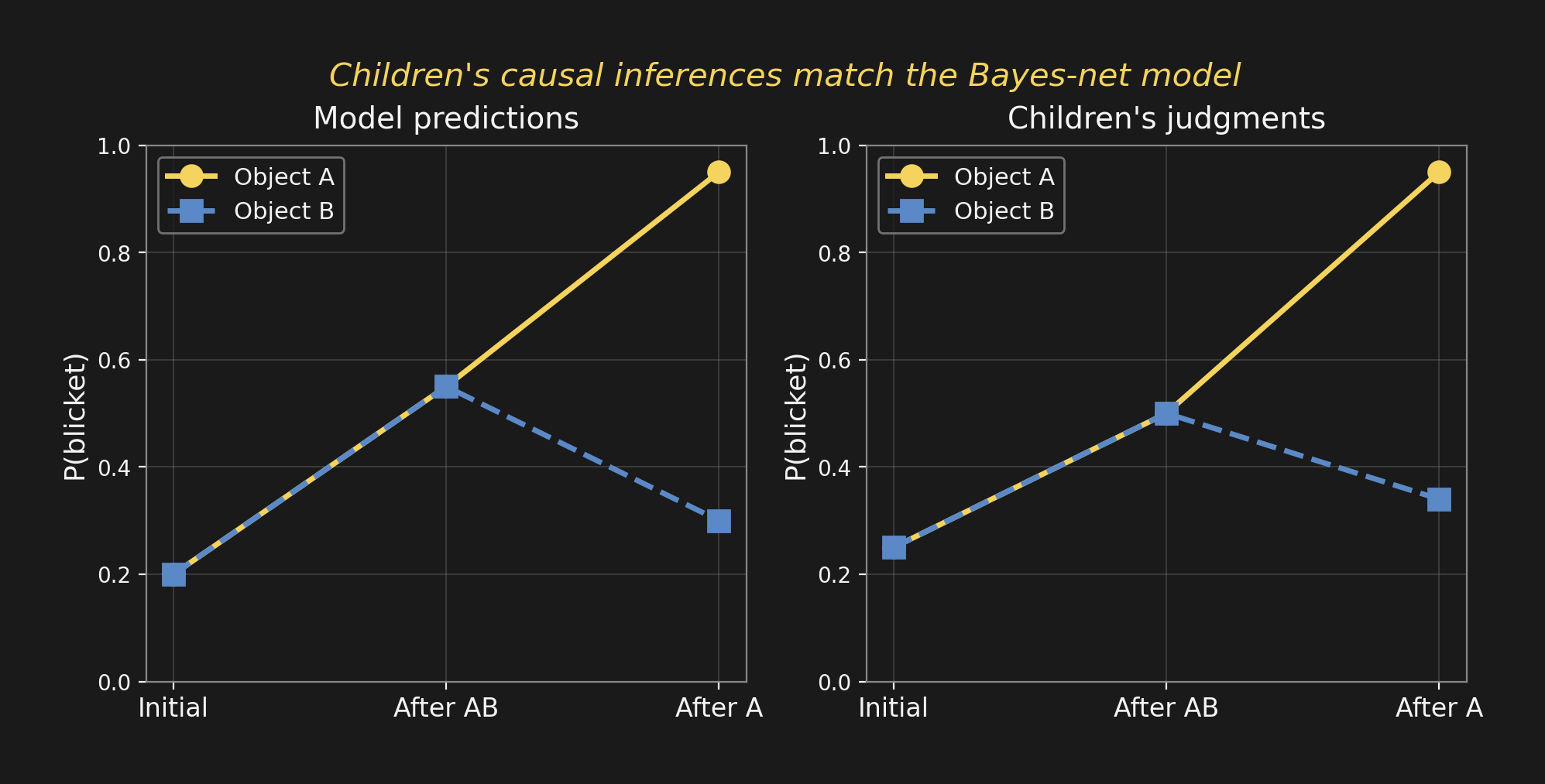
Children’s judgments drop for object B after the A-alone trial — even though nothing changed about B’s data. Children do graph surgery. They reason about the causal structure, not just statistical patterns.

The formal machinery isn’t just for engineers.

子どもの判断は、Aだけの試行のあとBについて 下がる — Bのデータについては 何も変わっていないのに。子どもはグラフ手術をしている。 統計パターンだけでなく、 因果構造について推論しているのです。

この形式的な仕組みは、エンジニアだけのものではありません。

~75 sec. Cog-sci payoff. By age 3-4, children are doing exactly the explaining-away reasoning we developed today. This is real cognition.

Did the prior come back?事前は戻ってくるか？

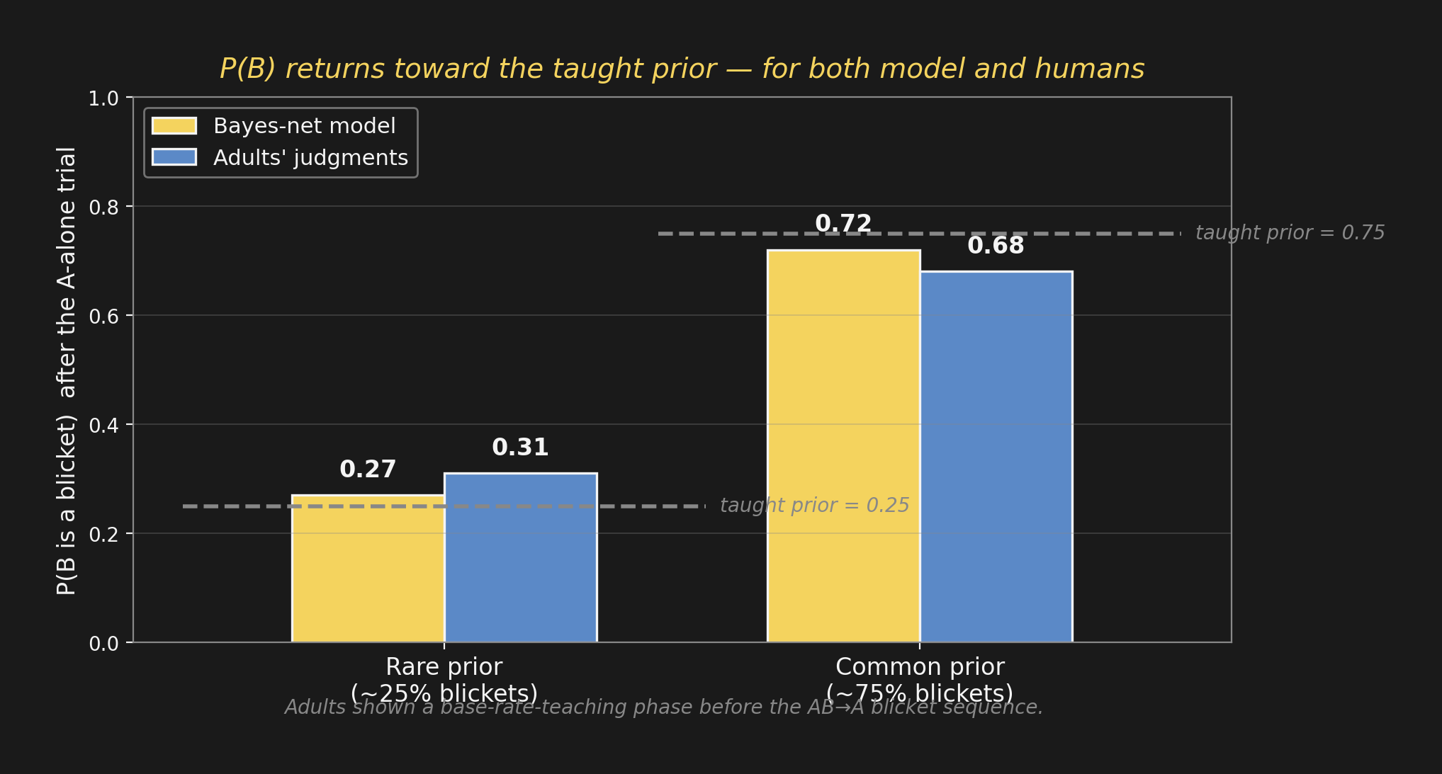
Design. Before the AB→A blicket sequence, adults watch a base-rate-teaching phase showing ~25% (“rare prior”) or ~75% (“common prior”) of arbitrary blocks are blickets. Then they run the classic backwards-blocking trials and rate \(P(B)\).

Bayes-net prediction. After A alone explains the AB result, the posterior on \(B\) should relax back toward the taught prior. Associative learning predicts a uniformly low rating regardless.

Result. Both the model AND adults snap \(P(B)\) back to the taught base rate — strong evidence that adults are reasoning Bayesianly over a causal graph, not just learning associations.

設計： AB→A の試行の前に、大人は「任意のブロックがブリケットである率」が ~25%（rare 事前）か ~75%（common 事前）かを学習する映像を見る。その後、定番の後方ブロッキング試行を行い \(P(B)\) を評価する。

ベイズネットの予測： A だけの試行が AB の結果を「説明」した後、\(B\) の事後分布は 教えられた事前に戻る。連合学習の予測は、教えた率に関係なく一律に低い評価。

結果： モデルも大人も \(P(B)\) を教えられた基準率に戻す — 大人は連合ではなく、因果グラフ上で ベイズ的に 推論している強い証拠。

~90 sec. THE prior-manipulation result. The classic Sobel/Tenenbaum/Gopnik backwards-blocking design with a taught base rate added before the AB→A trials. The discriminating test: after A explains the AB result, where does B’s posterior settle? Bayes net says “back to the prior you taught me”; associative learning predicts “uniformly low.” Humans match the Bayesian prediction across both conditions — same graph, two priors, two posterior landings. This is the strongest demo today that causal Bayes nets are the right cognitive model for adults, not just children.

Information theory + close情報理論 + まとめ

Entropy as expected surpriseエントロピー：期待される驚き

Define the surprise of seeing event \(X = x\) as

\[\text{surprise}(x) \;=\; \log \frac{1}{P(x)} \;=\; -\log P(x).\]

Smaller probability → larger surprise. The minus sign is there because \(\log P(x) \le 0\) when \(P(x) \le 1\), so \(-\log P(x) \ge 0\) — surprise is non-negative.

Event probability	Surprise (bits)
\(P(x) = 1\) (certain)	\(0\)
\(P(x) = 1/2\) (fair coin)	\(1\)
\(P(x) = 0.01\) (rare)	\(\approx 6.6\)

Entropy \(H(X)\) is the expected surprise:

\[H(X) \;=\; \sum_x P(x) \cdot \big[-\log P(x)\big] \;=\; \mathbb{E}\!\left[-\log P(X)\right].\]

事象 \(X = x\) を観測したときの 驚き を次のように定義する：

\[\text{驚き}(x) \;=\; \log \frac{1}{P(x)} \;=\; -\log P(x).\]

確率が小さいほど驚きが大きい。マイナス符号は、\(P(x) \le 1\) のとき \(\log P(x) \le 0\) なので、\(-\log P(x) \ge 0\) — 驚きが非負になるように。

事象の確率	驚き (ビット)
\(P(x) = 1\)（確実）	\(0\)
\(P(x) = 1/2\)（公正なコイン）	\(1\)
\(P(x) = 0.01\)（まれ）	\(\approx 6.6\)

エントロピー \(H(X)\) は驚きの 期待値：

\[H(X) \;=\; \sum_x P(x) \cdot \big[-\log P(x)\big] \;=\; \mathbb{E}\!\left[-\log P(X)\right].\]

~60 sec. Entropy = expected surprise. Surprise is -log(P). One sentence each for the three examples.

Mutual information相互情報量

How much does knowing \(Y\) reduce uncertainty about \(X\)? \[I(X; Y) \;=\; H(X) - H(X \mid Y)\]

Properties:

• \(I(X; Y) \geq 0\) always.
• \(I(X; Y) = 0 \iff X \perp Y\).
• \(I(X; Y) = I(Y; X)\) — symmetric.

Conditional version: \[I(X; Y \mid Z) = H(X \mid Z) - H(X \mid Y, Z).\] \(X \perp Y \mid Z\) iff \(I(X; Y \mid Z) = 0\).

\(Y\) を知ることは、\(X\) についての不確実性をどれだけ減らすか？ \[I(X; Y) \;=\; H(X) - H(X \mid Y)\]

性質：

• \(I(X; Y) \geq 0\) 常に。
• \(I(X; Y) = 0 \iff X \perp Y\)。
• \(I(X; Y) = I(Y; X)\) — 対称。

条件付き版： \[I(X; Y \mid Z) = H(X \mid Z) - H(X \mid Y, Z).\] \(X \perp Y \mid Z\) は \(I(X; Y \mid Z) = 0\) と同値。

~75 sec. The symmetry is the surprising property. Conditional MI is the bridge to today’s d-separation work.

The collider, in info-theoretic clothingコライダー、情報理論で

Take the Sprinkler / Rain / Wet-Grass collider:

• \(I(\text{Rain}; \text{Sprinkler}) = 0\) — independent a priori.
• \(I(\text{Rain}; \text{Sprinkler} \mid \text{Wet}) > 0\) — dependent after conditioning.

Conditioning on a collider creates mutual information from nothing.

That’s explaining away — viewed through a different lens. Info theory and Bayes nets are two languages describing the same structural facts.

スプリンクラー / 雨 / 濡れた芝生 のコライダーを考える：

• \(I(\text{雨}; \text{スプリンクラー}) = 0\) — 事前には独立。
• \(I(\text{雨}; \text{スプリンクラー} \mid \text{濡れた}) > 0\) — 条件付け後は従属。

コライダーへの条件付けは、無から相互情報量を生み出す。

これが説明はがし — 別の視点から見たもの。情報理論とベイズネットは、 同じ構造的事実を記述する2つの言語です。

~75 sec. THE punchline of the info-theory mini-block. Explaining away IS mutual-information creation. KL divergence gets a wordless forward pointer in next-week’s preview.

Next week — Week 6来週 — 第6週

Markov chains + networks. Random walks. Memory search.

Reading: Abbott, Austerweil & Griffiths (2012) — Human memory search as a random walk in a semantic network.

We’ve spent today on the structure of multi-variable distributions. Next week we walk on a network instead of conditioning on one.

マルコフ連鎖とネットワーク。 ランダムウォーク。記憶検索。

読み物: Abbott, Austerweil & Griffiths (2012) — Human memory search as a random walk in a semantic network.

今日はマルチ変数分布の 構造 について学びました。 来週はネットワークに条件付ける代わりに、その上を 歩く。

~30 sec. Hand-off. Two-week recap: this week was structure (conditional independence), next week is dynamics (random walks). DPMM is in the pre-read for context.

Thanksありがとうございました

Questions?

Office hours: by appointment. Slack me.

Reflections due before next Friday — pick any required or optional reading from this week. 5 of 11 across the semester.

質問は？

オフィスアワー：予約制。Slack でご連絡を。

リフレクションは次の金曜日までに — 今週の必須または推薦の読み物どれでもOK。 学期を通して 11 回中 5 回。

Close. Photo / icebreaker / Q&A as time permits.