Week 6 — Markov Chains + Networks第6週 — マルコフ連鎖とネットワーク

Friday, June 5, 20262026年6月5日（金）

Prof. Joseph Austerweilオウステウェイル　ジョセフ教授

Agenda本日の予定

• Welcome + a Markov chain you already knowようこそ + すでに知っているマルコフ連鎖 0:00
• Markov chains: states, transitions, the Markov propertyマルコフ連鎖：状態・遷移・マルコフ性 0:10
• Stationary distribution定常分布 0:25
• Networks: graphs as structureネットワーク：構造としてのグラフ 0:40
• Random walk on a networkネットワーク上のランダムウォーク 0:52
• Break休憩 1:07
• Memory search as a random walk (Abbott 2012)ランダムウォークとしての記憶探索（Abbott 2012） 1:12
• Network properties + PageRank + Week 7 bridgeネットワークの性質 + PageRank + 第7週へ 1:48

~2 min agenda. Today’s spine: ONE idea, built three times, each more concrete. (1) a Markov chain — states + a transition matrix; (2) a random walk on a network — a Markov chain whose states are nodes; (3) memory search — your own recall is a random walk on a semantic network (the required reading, Abbott 2012). Tell them: the thread connecting Week 5 (Bayes nets — directed graphs, the “Markov” factorization) to today is that we now add TIME. No presentation today; I cover the cognitive work myself. One break; polls throughout (the stationary-distribution examples and the degree result).

A Markov chain you already knowすでに知っているマルコフ連鎖

Block 1. Open with the phenomenon, let students react, THEN name it (show-before-tell). The Chibany bento chain. Also a one-slide admin note: Assignment 2 (Generalization) is due Jun 19 — point at the walkthrough page.

Admin — Assignment 2連絡 — 課題2

Assignment 2 (Generalization) is due Fri Jun 19, 8:00 PM — worth 7.5%.

• Build your own Bayesian generalization model: design a hypothesis space, then compute posteriors and predictions under weak vs. strong sampling.
• Walkthrough + stencils: hml.chibatech.dev/assignments.html — read the PDF first, then pick a stencil (GenJAX / Python / R), one-click “Open in Colab.”
• Reminder: 3 free late days pooled across the four programming assignments.
• Questions? DM me, or drop them in the class channel.

課題2（一般化）は6月19日（金）20:00締切 — 配点7.5%。

• 自分のベイズ一般化モデルを作る：仮説空間を設計し、弱い／強いサンプリングのもとで事後分布と予測を計算。
• 説明とひな形： hml.chibatech.dev/assignments.html — まずPDFを読み、ひな形（GenJAX／Python／R）を選んで「Open in Colab」を1クリック。
• 注意：4つのプログラミング課題で共通の無料遅延3日。
• 質問は DM か、クラスチャンネルへ。

~1.5 min. Assignment 2 = Generalization, due Jun 19 (7.5%). This is the natural week to point at it — it was assigned Week 4 and is now ~2 weeks out. Walk the assignments page briefly (PDF + three stencils + Colab), don’t re-derive the math. Questions go to me directly (DM) or the class channel — there is no dedicated #assignments channel. Then straight into Chibany.

Chibany’s bento habitチバニーのお弁当のクセ

New twist on Chibany this week: students now bring Chibany both a tonkatsu and a hamburger bento every day — and Chibany chooses which one to eat.

There’s a habit in the choosing: Chibany loves tonkatsu, so after a tonkatsu day they usually want it again — but every so often they fancy a change. And after a hamburger day, they almost always swing back to tonkatsu.

If Chibany chose tonkatsu yesterday, what will they probably eat today? And does it matter what they ate last Tuesday?

今週のチバニーの新展開： 学生は毎日チバニーに とんかつ と ハンバーグ の弁当を両方届けるようになり、チバニーがどちらを食べるか選ぶ。

選び方にクセがある：チバニーはとんかつが大好きなので、とんかつの日の翌日は たいていまたとんかつ — でもたまに気分を変えたくなる。そしてハンバーグの 日の翌日は、ほぼ必ずとんかつに戻る。

昨日チバニーがとんかつを選んだなら、今日はたぶん何を食べる? そして先週の火曜に何を食べたかは関係ある?

Show before tell. NOTE the deliberate narrative shift, called out in the dim line: in Weeks 1-2 students BROUGHT bentos and we did inference on the hidden contents (Chibany loves tonkatsu, 70/30 prior, opaque bentos). Here students bring BOTH a tonkatsu and a hamburger bento each day, and Chibany CHOOSES one — giving us an observable day-to-day SEQUENCE of choices, so we can study dependence over time. That’s what a Markov chain is about. Chibany uses they/them. Let 2-3 students answer out loud. The key thing to elicit: to guess today, you only need YESTERDAY — last Tuesday adds nothing once you know yesterday. That instinct IS the Markov property. Hold the name back one slide. ~2 min.

Draw the habitクセを図にする

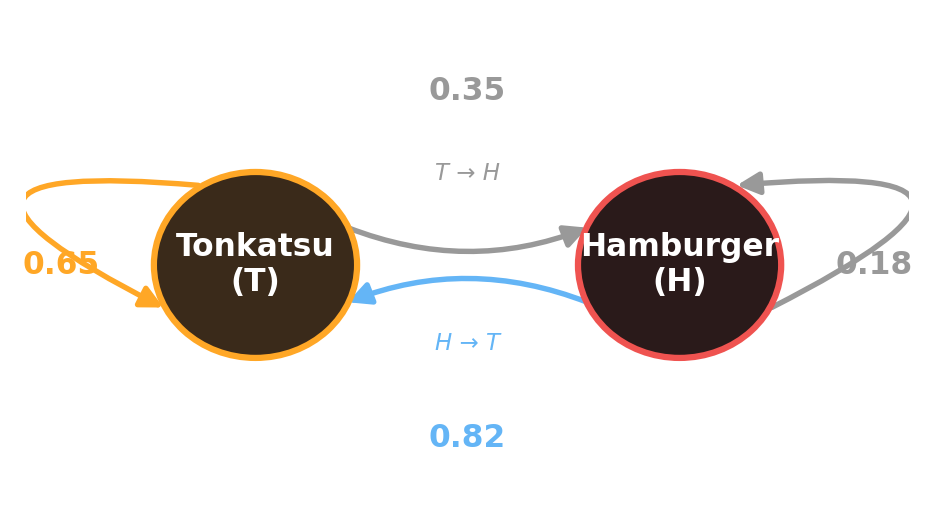
Two states (\(X_t\) = today’s bento), arrows = probabilities of tomorrow’s choice. Today depends only on yesterday. Chibany loves tonkatsu: sticks with it (0.65) and swings back to it after a burger (0.82).

2つの状態（\(X_t\) = 今日のお弁当）、矢印 = 明日の選択の確率。今日は昨日だけに依存する。チバニーはとんかつが大好き：とんかつを続け（0.65）、ハンバーグの後はとんかつに戻る（0.82）。

Introduce the symbol when you name the variable (CLAUDE.md rule): today’s bento is X_t, taking values T (tonkatsu) or H (hamburger). The transition probs are tuned so the STATIONARY distribution is 70% T / 30% H — matching Chibany’s canonical “loves tonkatsu, 70/30”. After tonkatsu: 0.65 stay, 0.35 switch. After hamburger: 0.82 back to tonkatsu, 0.18 repeat. Each row sums to 1. Don’t work the stationary math here — just note tonkatsu is “stickier”; it pays off in Block 3 when we compute the 70/30 stationary distribution. ~1 min.

Markovマルコフ

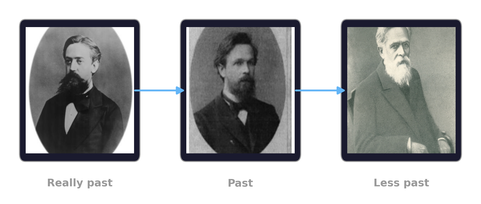
Given the present, the future is independent of the past.

現在を知れば、未来は過去と独立である。

The Andrey Markov “Really Past / Past / Less Past” gag (same mathematician, younger → older, left to right). The joke: it doesn’t matter HOW far back you go — once you know the present state, none of the past adds anything. This is the intuition for the Markov property BEFORE the formula on the next slide. The three photos are the actual SP25 deck images, composed into one figure so the captions align and arrows show the progression. ~1 min — land the yellow line, then formalize.

Name it: the Markov property名前をつける：マルコフ性

The future is independent of the past, given the present.

\[P(X_{t+1} \mid X_t, X_{t-1}, \dots, X_0) \;=\; P(X_{t+1} \mid X_t)\]

• Once you know today (\(X_t\)), the whole earlier history tells you nothing more about tomorrow.
• A sequence with this property is a Markov chain.

現在を知れば、未来は過去と独立である。

\[P(X_{t+1} \mid X_t, X_{t-1}, \dots, X_0) \;=\; P(X_{t+1} \mid X_t)\]

• 今日（\(X_t\)）さえ分かれば、それより前の履歴は明日について何も追加情報を与えない。
• この性質を持つ系列をマルコフ連鎖と呼ぶ。

This is the definition. “Really Past / Past / Less Past” — none of it matters once you have the present. Connect to Week 5: there we drew directed graphs (Bayes nets) and used the word “Markov” for the factorization. Here it’s the same independence idea, but indexed by TIME. ~2 min.

Where we are現在地

• Welcome + a Markov chain you already knowようこそ + すでに知っているマルコフ連鎖 0:00
• Markov chains: states, transitions, the Markov propertyマルコフ連鎖：状態・遷移・マルコフ性 0:10
• Stationary distribution定常分布 0:25
• Networks: graphs as structureネットワーク：構造としてのグラフ 0:40
• Random walk on a networkネットワーク上のランダムウォーク 0:52
• Break休憩 1:07
• Memory search as a random walk (Abbott 2012)ランダムウォークとしての記憶探索（Abbott 2012） 1:12
• Network properties + PageRank + Week 7 bridgeネットワークの性質 + PageRank + 第7週へ 1:48

Recap ~10s. Chibany set up the idea; now formalize states + transition matrix.

Markov chains: the machineryマルコフ連鎖：仕組み

Block 2. States, the transition matrix, two views (FSA + matrix), card shuffle.

Notation lock-in記号の確認

• \(X_t\) — the state at time \(t\) (one of a finite set \(\mathcal{S}\)). Chibany: \(X_t \in \{\text{T}, \text{H}\}\).
• \(P\) — the transition matrix: \(P_{ij} = P(X_{t+1}=j \mid X_t=i)\).
• \(\pi\) — the stationary distribution (the long-run fractions — defined fully next segment).

Each row of \(P\) is a probability distribution over next states → it sums to 1. Such a matrix is called row-stochastic.

• \(X_t\) — 時刻 \(t\) の状態（有限集合 \(\mathcal{S}\) の1つ）。チバニー: \(X_t \in \{\text{T}, \text{H}\}\)。
• \(P\) — 遷移行列: \(P_{ij} = P(X_{t+1}=j \mid X_t=i)\)。
• \(\pi\) — 定常分布（長期的な割合 — 次のセグメントで完全に定義）。

\(P\) の各行は次状態の確率分布 → 合計1。このような行列を行確率的と呼ぶ。

Define before use. The row-sums-to-1 point matters — it’s why P^k stays a valid distribution and why the largest eigenvalue is 1. Name pi now so next segment’s formula has nothing to decode. ~2 min.

Two views of the same chain同じ連鎖の2つの見方

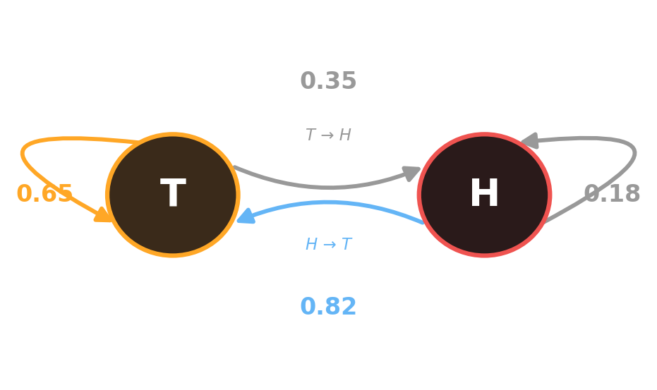
Picture view: Chibany’s chain — states + labeled arrows (the same one from “Draw the habit”).

絵の見方： チバニーの連鎖 — 状態 + ラベル付き矢印（「クセを図にする」と同じもの）。

Matrix view: \[P = \begin{pmatrix} 0.65 & 0.35 \\ 0.82 & 0.18 \end{pmatrix}\]

Row 1 = “if T today, then tomorrow.” Row 2 = “if H today.” (columns are T, H)

Same chain, two pictures.

行列の見方： \[P = \begin{pmatrix} 0.65 & 0.35 \\ 0.82 & 0.18 \end{pmatrix}\]

行1 =「今日 T なら、明日は」。行2 =「今日 H なら」。 （列は T, H）

同じ連鎖、2つの絵。

The picture and the matrix are the SAME object. Two-column because there’s genuine structural parallelism. Next slide shows how the matrix actually generates a step — the seed of Monte Carlo at the end. ~2 min.

The matrix is a sampler行列はサンプラー

How does the chain actually take a step? You roll a (continuous) die.

Say today is tonkatsu (T), so the row is \([\,0.65,\; 0.35\,]\) — 0.65 stay T, 0.35 switch to H.

1. Draw a random number \(u\) evenly between 0 and 1. (Say \(u = 0.42\).)
2. \(0.42 < 0.65\) → stay at T. (If it were \(> 0.65\) → switch to H.)

Repeat tomorrow, and the next day… the matrix plus a stream of random numbers generates the whole sequence. Hold this idea — it returns at the end of class.

連鎖は実際にどう1歩進む? （連続的な）サイコロを振る。

今日が とんかつ (T) なら、行は \([\,0.65,\; 0.35\,]\) — 0.65でT継続、0.35でHへ。

1. 0と1の間で一様な乱数 \(u\) を引く。（例：\(u = 0.42\)。）
2. \(0.42 < 0.65\) → Tに留まる。（\(> 0.65\) なら → Hへ切替。）

翌日も、その次の日も繰り返す… 行列 + 乱数の流れが系列全体を生成する。 この発想を覚えておいて — 授業の最後に戻ってくる。

This is the slide the student review asked for: give the uniform-draw its own concrete micro-example (u=0.73 > stay) instead of cramming it onto the two-views slide. “Roll a continuous die” is the intuition for Uniform(0,1). This is the explicit seed of Monte Carlo — called back on the bridge slide. ~2 min.

Run it: what a chain produces動かす：連鎖が生み出すもの

Five runs of Chibany’s chain, each starting at T:

T H T H T T H T H T T T H T H T T T T H
T T H T H H T T T T T H T H T T T T T T
T T H T H T T H T T T H T T T H T H T T
T T T T H T T H T T T T T T T T H T T T
T T H T H T T H T T T H T T T T H T T T

Mostly T, with brief H interruptions (hamburger almost never repeats). Over time, roughly 70% T, 30% H.

チバニーの連鎖を5回走らせる。各回 T から開始：

T H T H T T H T H T T T H T H T T T T H
T T H T H H T T T T T H T H T T T T T T
T T H T H T T H T T T H T T T H T H T T
T T T T H T T H T T T T T T T T H T T T
T T H T H T T H T T T H T T T T H T T T

ほとんど T、たまに H が割り込む（ハンバーグはほぼ繰り返さない）。長い目で見ると、おおよそ 70% T, 30% H。

Real samples from Chibany’s chain (T->T .65, H->T .82). The point: the chain has memory-of-one-step (you see T tends to persist, H flips right back), yet a stable long-run frequency emerges — ~70% T. That long-run frequency is the stationary distribution, which we make precise next segment AND compute as 70/30. ~2 min.

Where we are現在地

• Welcome + a Markov chain you already knowようこそ + すでに知っているマルコフ連鎖 0:00
• Markov chains: states, transitions, the Markov propertyマルコフ連鎖：状態・遷移・マルコフ性 0:10
• Stationary distribution定常分布 0:25
• Networks: graphs as structureネットワーク：構造としてのグラフ 0:40
• Random walk on a networkネットワーク上のランダムウォーク 0:52
• Break休憩 1:07
• Memory search as a random walk (Abbott 2012)ランダムウォークとしての記憶探索（Abbott 2012） 1:12
• Network properties + PageRank + Week 7 bridgeネットワークの性質 + PageRank + 第7週へ 1:48

Recap ~10s. We’ve seen a chain produce long-run frequencies (Chibany ~70% T). Now make “long-run frequency” precise: the stationary distribution. Open the segment with card shuffling to motivate the GOAL.

The stationary distribution定常分布

Block 3. Open with card shuffling (process → goal), THEN the long-run question; pi P = pi; find it by power iteration; the “start doesn’t matter” poll; name the eigenvector fact (no PCA/SVD aside).

Shuffling a deckデッキをシャッフルする

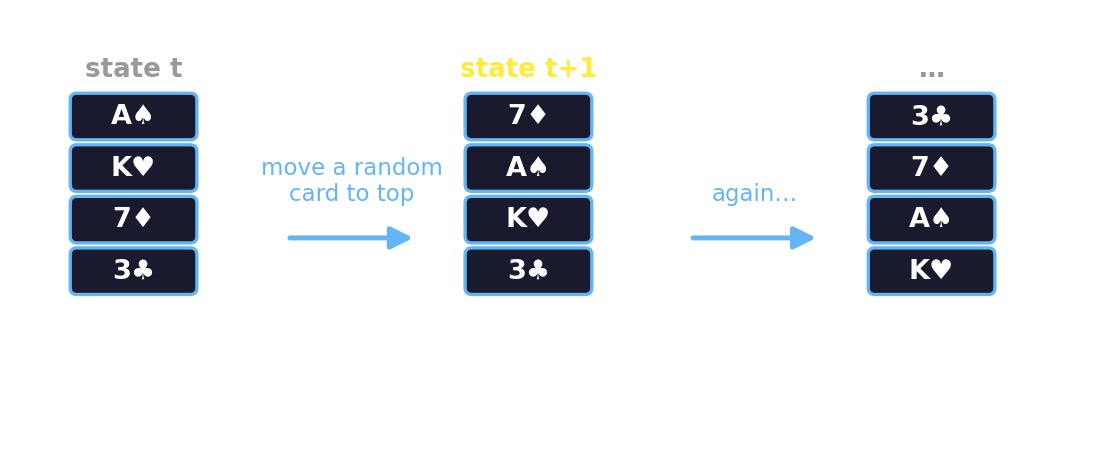
• State = the deck’s current ordering
• Transition = “move a random card to the top,” over and over

You shuffle a deck before a game. What are you actually trying to achieve — what’s the computational goal of shuffling?

• 状態 = デッキの現在の並び
• 遷移 =「ランダムなカードを一番上へ」を繰り返す

ゲームの前にデッキをシャッフルする。本当は何を達成しようとしている — シャッフルの計算的なゴールは?

This is the SEGMENT OPENER for stationary distributions — process only, no “stationary” word yet. Card shuffling is a Markov chain (state = ordering, transition = move-random-card-to-top). Ask the question and let students answer out loud: “what’s the goal of shuffling?” Steer toward: make every ordering equally likely / no ordering predictable / fair. Hold the formal answer for the NEXT slide. ~1.5 min. (Don’t say “stationary distribution” yet.)

The goal: a distribution that stops changingゴール：変わらなくなる分布

The goal of shuffling: make every ordering equally likely — a uniform distribution over all \(52!\) orderings.

• Shuffle once more from there, and the distribution is still uniform — shuffling can’t make it “more shuffled.”
• That self-perpetuating, no-longer-changing distribution is what this whole lecture segment is about.

We were never after one ordering — we were after a distribution the process settles into. Let’s make that precise.

シャッフルのゴール：すべての並びを等確率にする — \(52!\) 通りの並びに対する一様分布。

• そこからもう一度シャッフルしても、分布はまだ一様 — それ以上「シャッフル」できない。
• この自己保存的でもう変わらない分布こそ、このセグメント全体のテーマ。

私たちは1つの並びを求めていたのではない — 過程が落ち着く分布を求めていた。これを正確にしよう。

The reveal/payoff of the shuffling question, and the bridge INTO the formal definition. The goal of shuffling = uniform over orderings, and crucially: once you’re there, shuffling keeps you there (it stops changing). That “stops changing” property IS stationarity — which we name on the next slide. 52! is astronomically large, so you can’t compute it by listing orderings; you reach it by RUNNING the process. Foreshadows power iteration. ~1.5 min.

The long-run question長期の問い

Run a chain for a very long time. What fraction of the time do you spend in each state?

Over a whole semester, what fraction of Chibany’s lunches are tonkatsu?

Call that distribution \(\pi\).

Definition: \(\pi\) is stationary if running one more step doesn’t change it: \[\pi P = \pi\]

If you’re already distributed as \(\pi\), you stay distributed as \(\pi\) forever.

連鎖を非常に長く走らせる。各状態で過ごす時間の割合は?

1学期を通して、チバニーの昼食のうちとんかつは何割?

その分布を \(\pi\) と呼ぶ。

定義： もう1歩進めても変わらないとき \(\pi\) は定常： \[\pi P = \pi\]

すでに \(\pi\) の分布なら、その後ずっと \(\pi\) のまま。

State it; don’t derive it. pi P = pi: a fixed point of the chain’s dynamics. Anchor with Chibany: his chain (0.65/0.35, 0.82/0.18) settles to pi = 70% tonkatsu / 30% hamburger — exactly the 70/30 “loves tonkatsu” prior students saw in Week 2. The coin’s pi was (1/2, 1/2); the shuffle’s was uniform over orderings. Question now: how do we FIND pi for a chain we’re handed? Two answers — run it (power iteration, this segment) or solve the eigen-equation (the assignment). ~2 min.

How to find π — just run itπ の求め方 — とにかく走らせる

Start from any distribution and step repeatedly — i.e. multiply by \(P\) over and over: \[\mathbf{v},\; \mathbf{v}P,\; \mathbf{v}P^2,\; \mathbf{v}P^3,\; \dots \;\longrightarrow\; \pi\]

This is called power iteration. Let’s watch it on Chibany’s chain.

任意の分布から始めて、繰り返し1歩進める — つまり \(P\) を何度も掛ける： \[\mathbf{v},\; \mathbf{v}P,\; \mathbf{v}P^2,\; \mathbf{v}P^3,\; \dots \;\longrightarrow\; \pi\]

これをべき乗法と呼ぶ。チバニーの連鎖で見てみよう。

Set up the build-up that follows, on the SAME Chibany chain we’ve used all along (0.65/0.35, 0.82/0.18). Poll FIRST (before the figure), then reveal. ~1 min.

Poll — does the start matter?ポール — 出発点は関係ある?

We’ll run Chibany’s chain two ways — he always starts on tonkatsu, or always on hamburger — for 20 days.

Before we look: is the chance he’s eating tonkatsu on day 20 the same either way?

チバニーの連鎖を2通りで走らせる — いつもとんかつから始める、またはいつもハンバーグから — 20日間。

見る前に： 20日目にとんかつを食べている確率は、どちらから始めても同じ?

• A. essentially the same
• B. clearly different — the start sticks
• C. it depends on the exact matrix

• A. ほぼ同じ
• B. 明らかに違う — 出発点が残る
• C. 行列次第

COMMIT BEFORE REVEAL — this poll comes BEFORE the convergence figure, so students actually have to predict. Don’t show the figure yet. The same “does the start matter?” question is the SP25 “Markov chains and networks” quiz Q4; we hit it again on the 3-state example. ~1 min, then reveal on the next slide.

Two different starts — the reveal2つの異なる出発点 — 答え合わせ

Same start always-tonkatsu (top) vs always-hamburger (bottom). After \(k\) steps:

いつもとんかつから（上）対 いつもハンバーグから（下）。\(k\)ステップ後：

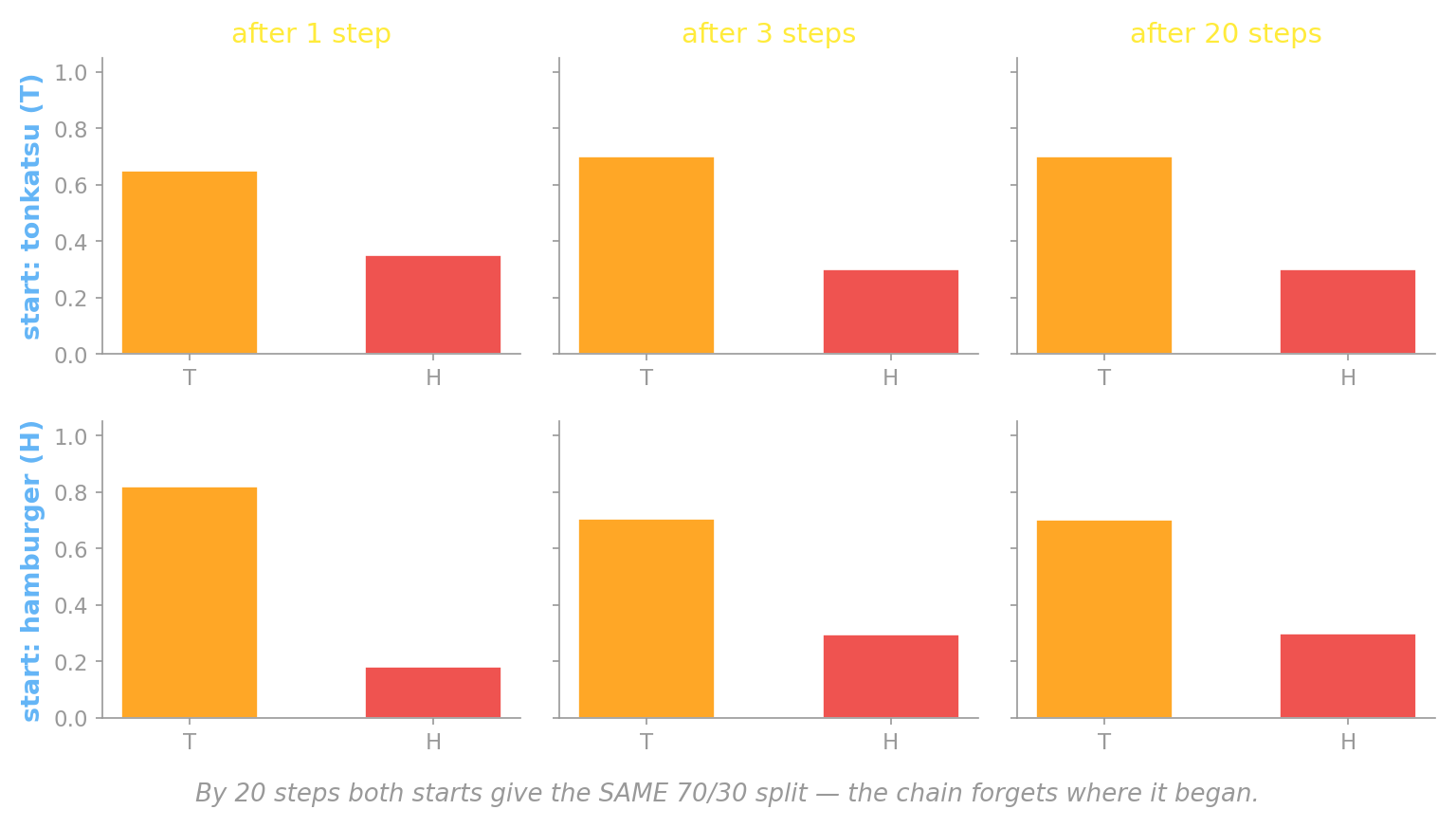
A. Essentially the same. After 1 step they differ; by 20 steps both reach 70% T / 30% H. The chain forgot where it started.

A. ほぼ同じ。 1ステップ後は違うが、20ステップで両方とも 70% T / 30% H に到達。連鎖は出発点を忘れた。

THE reveal of the poll. Top row starts always-tonkatsu, bottom always-hamburger. After 1 step they look different; by 20 steps both rows are IDENTICAL — 70/30 — the chain forgot its start. That common distribution is Chibany’s stationary pi. ~2 min. The “why” (ergodicity) is the next slide.

Why? The chain mixesなぜ? 連鎖は混合する

After enough days the chain forgets where it started — it mixes. The long-run distribution is the stationary \(\pi\) (Chibany’s 70/30), and (for a well-behaved chain) it’s the same from every starting point.

The technical condition is ergodicity — you can get from any state to any other, and the chain doesn’t get trapped in a cycle.

十分な日数の後、連鎖は出発点を忘れる — 混合する。長期の分布は 定常分布 \(\pi\) であり、（性質の良い連鎖では）どの出発点からでも同じ。

技術的条件はエルゴード性 — どの状態からどの状態へも到達でき、周期に 閉じ込められないこと。

The “why” behind the poll answer. Define ergodicity in one dim line — get-anywhere + not-periodic. Don’t prove it. The takeaway: pi is a property of the chain, not of where you start. ~1.5 min.

Where does π come from?π はどこから来る?

Power iteration converges to \(\pi\). But what is \(\pi\), exactly?

\(\pi\) is the left eigenvector of \(P\) with eigenvalue 1.

• An eigenvector of a matrix is a vector whose direction is unchanged when you multiply by the matrix — only its length scales, by a factor called the eigenvalue.
• Since \(\pi P = \pi\) (unchanged, scale \(=1\)), \(\pi\) is exactly the eigenvector with eigenvalue 1. Every row-stochastic matrix has one.

The bar charts showed this: once the shape stopped changing under \(\times P\), you’d found \(\pi\).

べき乗法は \(\pi\) に収束する。では \(\pi\) とは正確には何?

\(\pi\) は 固有値1に対応する \(P\) の左固有ベクトル。

• 行列の固有ベクトルとは、その行列を掛けても方向が変わらないベクトル — 長さだけが固有値という倍率で変わる。
• \(\pi P = \pi\)（不変、倍率 \(=1\)）なので、\(\pi\) はまさに固有値1の固有ベクトル。行確率行列は必ず1つ持つ。

棒グラフが示したこと：\(\times P\) で形が変わらなくなったら \(\pi\) を見つけた。

State the eigenvector fact in ONE slide; define eigenvector in one line. Do NOT bring in PCA/SVD (the SP25 aside is deliberately cut — it derails the process narrative and most SDS students are shaky on it). The explicit eigen-solve is in the assignment, not the lecture. The lecture route is power iteration; the eigenvector is the “what it converges to” footnote. ~2 min.

Now try a harder one — togetherもう少し難しいのを — 一緒に

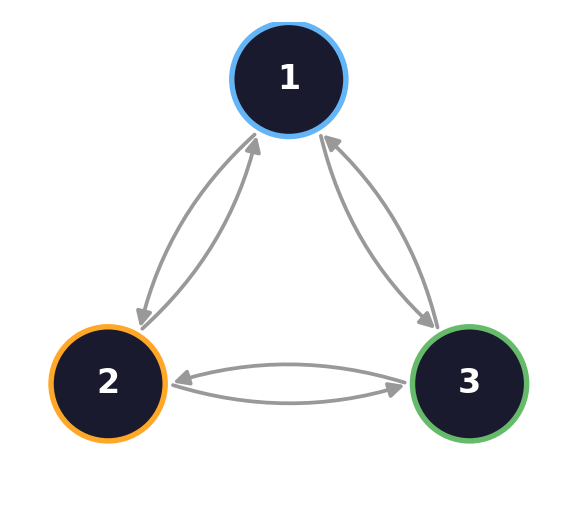
A 3-state random walk (states 1, 2, 3). Same rules as Chibany — just more states. Its transition matrix:

\[A = \begin{pmatrix} 0 & 0.1 & 0.9 \\ 0.5 & 0 & 0.5 \\ 0.8 & 0.2 & 0 \end{pmatrix}\]

Row \(i\) = where you go from state \(i\). (No self-loops here — the diagonal is 0.)

3状態のランダムウォーク（状態 1, 2, 3）。チバニーと同じルール — 状態が増えただけ。遷移行列：

\[A = \begin{pmatrix} 0 & 0.1 & 0.9 \\ 0.5 & 0 & 0.5 \\ 0.8 & 0.2 & 0 \end{pmatrix}\]

行 \(i\) = 状態 \(i\) からの行き先。（ここでは自己ループなし — 対角は0。）

The SECOND worked example, fully presented (the SP25 “Markov chains and networks” quiz matrix). Goal: show the SAME machinery — power iteration → stationary π — generalizes beyond the 2-state Chibany chain. Read the matrix together: from state 1 you go to 2 w.p. 0.1 or to 3 w.p. 0.9, etc. Then poll intuitions BEFORE computing. ~1.5 min.

Poll — guess before we computeポール — 計算する前に予想

\[A = \begin{pmatrix} 0 & 0.1 & 0.9 \\ 0.5 & 0 & 0.5 \\ 0.8 & 0.2 & 0 \end{pmatrix}\]

Run this 3-state walk a long time. Which state does it visit MOST often?

Which state do the others tend to send you toward?

• A. state 1
• B. state 2
• C. state 3
• D. all about equal

この3状態のウォークを長く走らせる。最も頻繁に訪れる状態は?

他の状態はどこへ送りがち?

• A. 状態1
• B. 状態2
• C. 状態3
• D. ほぼ均等

Commit before reveal — this tests intuition, and the network + matrix are RIGHT THERE so students can reason. The clue: state 1 sends 0.9 to state 3, state 2 sends 0.5 to state 3 — lots of arrows point at 3 (and at 1). State 2 is rarely a destination (only 0.1 from 1, 0.2 from 3). So 1 and 3 high, 2 low. Don’t reveal exact numbers yet — compute them next. ~1 min.

Work it out — power iteration計算する — べき乗法

Same method as Chibany: pick two starts (state 1 / state 2), multiply by \(A\) over and over.

チバニーと同じ方法：2つの出発点（状態1 / 状態2）を選び、\(A\) を何度も掛ける。

Work the power iteration live or step through the figure. Top row starts in state 1, bottom in state 2. After 1 step: very different. By 20 steps: identical — and state 2 is clearly the smallest, states 1 and 3 nearly tied, as the poll intuition predicted. ~2 min.

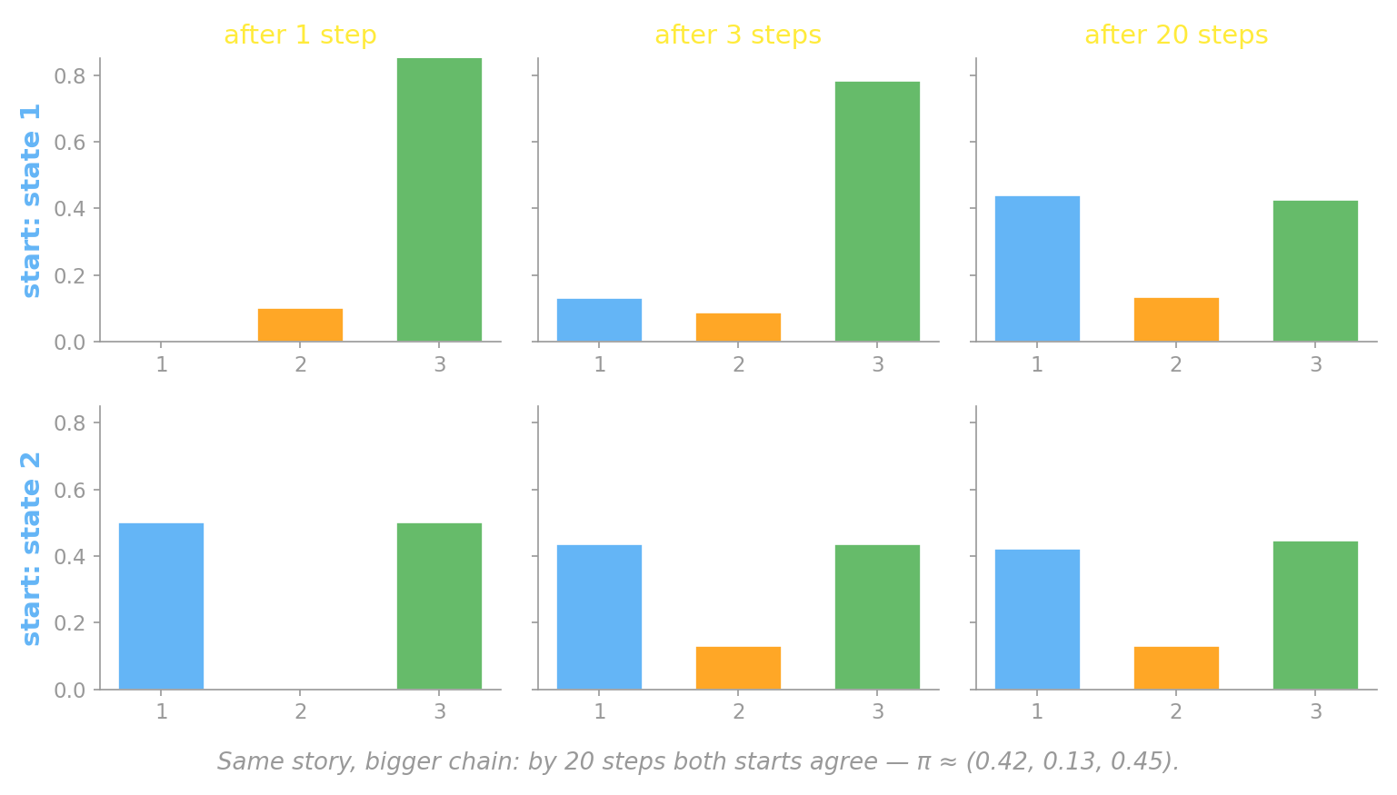
Poll — does the start matter? (again)ポール — 出発点は関係ある?（再び）

\[A = \begin{pmatrix} 0 & 0.1 & 0.9 \\ 0.5 & 0 & 0.5 \\ 0.8 & 0.2 & 0 \end{pmatrix}\]

Run this walk for 20 steps. Is the chance of being in state 2 the same from state 1 as from state 2?

Same question we asked for Chibany — does it still hold with 3 states?

• A. essentially the same
• B. clearly different
• C. depends on the matrix

このウォークを20ステップ走らせる。状態2にいる確率は、状態1からでも状態2からでも同じ?

チバニーで聞いたのと同じ問い — 3状態でも成り立つ?

• A. ほぼ同じ
• B. 明らかに違う
• C. 行列次第

SP25 “Markov chains and networks” quiz Q2 vs Q3 → Q4, now as a poll on the matrix it was actually written for. Answer: A — same (~0.13 either way). The chain is ergodic, so it forgets its start regardless of how many states. ~1 min.

The 3-state stationary distribution3状態の定常分布

A. Essentially the same — and the walk’s long-run home is:

\[\pi \approx (\,0.42,\; 0.13,\; 0.45\,)\]

• States 1 and 3 soak up most of the visits (everyone points toward them).
• State 2 is rarely visited — exactly the poll intuition.
• Two states, three states, or 52! card orderings — same method, same kind of answer.

A. ほぼ同じ — そしてウォークの長期的な居場所は：

\[\pi \approx (\,0.42,\; 0.13,\; 0.45\,)\]

• 状態1と3がほとんどの訪問を集める（皆そこを指す）。
• 状態2はめったに訪れない — まさに予想どおり。
• 2状態、3状態、あるいは 52! 通りのカードの並び — 同じ方法、同じ種類の答え。

The payoff: the machinery generalizes. pi ≈ (0.42, 0.13, 0.45) — states 1 and 3 dominate, state 2 is rare, matching the pre-compute poll. Tie it together: the same power-iteration → stationary recipe worked for Chibany (2 states), this walk (3 states), and the card shuffle (52! states). The assignment has them solve the stationary distribution explicitly (eigenvector) for this exact matrix. ~1.5 min.

Where we are現在地

• Welcome + a Markov chain you already knowようこそ + すでに知っているマルコフ連鎖 0:00
• Markov chains: states, transitions, the Markov propertyマルコフ連鎖：状態・遷移・マルコフ性 0:10
• Stationary distribution定常分布 0:25
• Networks: graphs as structureネットワーク：構造としてのグラフ 0:40
• Random walk on a networkネットワーク上のランダムウォーク 0:52
• Break休憩 1:07
• Memory search as a random walk (Abbott 2012)ランダムウォークとしての記憶探索（Abbott 2012） 1:12
• Network properties + PageRank + Week 7 bridgeネットワークの性質 + PageRank + 第7週へ 1:48

Recap ~10s. We have chains + stationary distributions in the abstract. Now give the states STRUCTURE: make them nodes of a network.

Networks: graphs as structureネットワーク：構造としてのグラフ

Block 4. Networks as graphs; from a graph to a transition matrix (the hinge); then Block 5 walks on it.

What’s a graph?グラフとは?

A graph \(G = (V, E)\) is just nodes (\(V\)) joined by edges (\(E\)).

• Edges can be undirected (mutual) or directed (one-way)
• Edges can be weighted (stronger / weaker)

You already met graphs last week — a Bayes net is a directed graph. There an edge meant “depends on”; the graphs today use edges to mean “is related / connected to.”

グラフ \(G = (V, E)\) とは、ノード（\(V\)）をエッジ（\(E\)）で結んだもの。

• エッジは無向（相互）または有向（一方向）
• エッジは重み付きにできる（強弱）

グラフは先週すでに登場した — ベイズネットは有向グラフ。そこでのエッジは「依存する」の意味だったが、今日のグラフではエッジは「関連・接続している」を意味する。

Introduce the graph abstraction generically FIRST, and anchor it to last week: a Bayes net IS a directed graph (nodes = variables, edges = “depends on”). Today the same object, edges meaning “related/connected.” ~1.5 min. Examples next.

Graphs are everywhereグラフはどこにでもある

The power of the abstraction: one object, many domains. What are the nodes and edges?

抽象化の力：1つの対象、多くの領域。 ノードとエッジは何?

Graph	Nodes	Edges
Semantic network (cog sci)	concepts / words	“is related / associated”
The Web	web pages	hyperlinks (directed)
Co-authorship network	researchers	“wrote a paper together”
Social network	people	friendships / follows
Road map	intersections	roads (weighted = distance)
Neural network (brain)	neurons	synapses

Today’s star is the semantic network — concepts as nodes, associations as edges. Cognitive science has used it for decades (Collins & Quillian 1969; Collins & Loftus 1975).

グラフ	ノード	エッジ
意味ネットワーク（認知科学）	概念 / 単語	「関連・連想する」
ウェブ	ウェブページ	ハイパーリンク（有向）
共著ネットワーク	研究者	「一緒に論文を書いた」
ソーシャルネットワーク	人	友人関係 / フォロー
道路地図	交差点	道路（重み = 距離）
神経回路（脳）	ニューロン	シナプス

今日の主役は意味ネットワーク — 概念がノード、連想がエッジ。認知科学は何十年も使ってきた（Collins & Quillian 1969; Collins & Loftus 1975）。

The “one abstraction, many domains” slide. Each row makes nodes/edges explicit so the abstraction is concrete. The Web row foreshadows PageRank (segment 8); the semantic-network row is the one we build on (the Abbott payoff). Co-authorship + social are familiar to students. ~2 min. Land: today we walk on the semantic network.

The graph as a matrix行列としてのグラフ

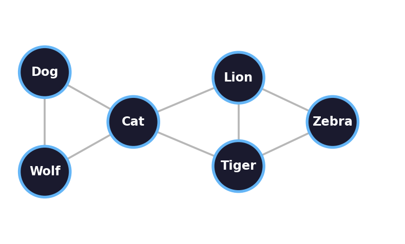
Adjacency matrix \(L\): \(L_{ij} = 1\) when nodes \(i\) and \(j\) share an edge, else \(0\).

\[L = \begin{array}{r|cccccc} & \text{D} & \text{W} & \text{C} & \text{L} & \text{T} & \text{Z} \\ \hline \text{Dog} & 0 & 1 & 1 & 0 & 0 & 0 \\ \text{Wolf} & 1 & 0 & 1 & 0 & 0 & 0 \\ \text{Cat} & 1 & 1 & 0 & 1 & 1 & 0 \\ \text{Lion} & 0 & 0 & 1 & 0 & 1 & 1 \\ \text{Tiger} & 0 & 0 & 1 & 1 & 0 & 1 \\ \text{Zebra} & 0 & 0 & 0 & 1 & 1 & 0 \end{array}\]

Symmetric (undirected). Each row sum = that node’s degree — Cat’s row sums to 4.

隣接行列 \(L\)：ノード \(i\) と \(j\) がエッジで繋がっていれば \(L_{ij} = 1\)、なければ \(0\)。

\[L = \begin{array}{r|cccccc} & \text{D} & \text{W} & \text{C} & \text{L} & \text{T} & \text{Z} \\ \hline \text{Dog} & 0 & 1 & 1 & 0 & 0 & 0 \\ \text{Wolf} & 1 & 0 & 1 & 0 & 0 & 0 \\ \text{Cat} & 1 & 1 & 0 & 1 & 1 & 0 \\ \text{Lion} & 0 & 0 & 1 & 0 & 1 & 1 \\ \text{Tiger} & 0 & 0 & 1 & 1 & 0 & 1 \\ \text{Zebra} & 0 & 0 & 0 & 1 & 1 & 0 \end{array}\]

対称（無向）。各行の和 = そのノードの次数 — Cat の行は4。

The explicit adjacency matrix L for the animal network, shown large beside the graph so students see the graph↔︎matrix correspondence concretely. Point out one or two entries: L[Cat,Lion]=1 because there’s an edge; L[Dog,Lion]=0 because there isn’t. Symmetric because undirected. Row sums = degrees (Cat=4, the hub). Next slide: normalize rows → transition matrix P. ~2 min.

From a graph to a transition matrixグラフから遷移行列へ

The hinge of the whole lecture:

1. List the edges in an adjacency matrix \(L\): \(L_{ij} = 1\) if \(i\)–\(j\) are connected (or a positive weight).
2. Normalize each row to sum to 1 → a transition matrix \(P\).

Now \(P\) describes a walker who, at each node, steps to a random neighbor.

Structure (the graph) + process (the walk) — a Markov chain whose states are nodes.

講義全体の要：

1. エッジを隣接行列 \(L\) に並べる：\(i\)–\(j\) が繋がっていれば \(L_{ij} = 1\)（または正の重み）。
2. 各行を正規化して合計1に → 遷移行列 \(P\)。

\(P\) は、各ノードでランダムな隣へ進む歩行者を表す。

構造（グラフ） + 過程（ウォーク） — 状態がノードであるマルコフ連鎖。

THIS is the hinge that turns Block 4’s structure into Block 2’s process. Row- normalize the adjacency matrix and you have a random walk. Two-column: graph on the left, the recipe on the right. ~3 min.

Where we are現在地

• Welcome + a Markov chain you already knowようこそ + すでに知っているマルコフ連鎖 0:00
• Markov chains: states, transitions, the Markov propertyマルコフ連鎖：状態・遷移・マルコフ性 0:10
• Stationary distribution定常分布 0:25
• Networks: graphs as structureネットワーク：構造としてのグラフ 0:40
• Random walk on a networkネットワーク上のランダムウォーク 0:52
• Break休憩 1:07
• Memory search as a random walk (Abbott 2012)ランダムウォークとしての記憶探索（Abbott 2012） 1:12
• Network properties + PageRank + Week 7 bridgeネットワークの性質 + PageRank + 第7週へ 1:48

Recap ~10s. We can turn any graph into a chain. Now WALK it — and watch what the walk visits.

Random walk on a networkネットワーク上のランダムウォーク

Block 5. The Meow/Cat/Dog walk build-up; the degree result; the degree poll.

Take a walk — step 1歩いてみる — ステップ1

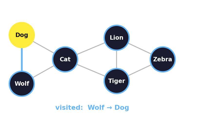
Start at Wolf. Pick a random neighbor → Dog.

The sequence of nodes we visit is a Markov chain.

Wolf から開始。ランダムな隣を選ぶ → Dog。

訪れるノードの系列がまさにマルコフ連鎖。

Build-up as sibling slides (not fragments) — each step its own slide, so it reads as animation. Step 1: Wolf -> Dog. ~20s per slide. Highlighted node = where the walker is now; blue edges = the path so far.

Take a walk — step 2歩いてみる — ステップ2

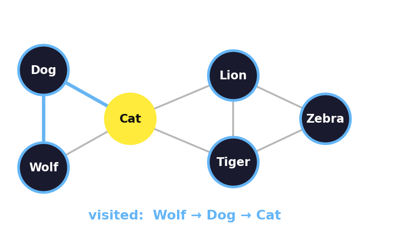
Dog → random neighbor → Cat.

Dog → ランダムな隣 → Cat。

Step 2: Dog -> Cat (into the bridge node).

Take a walk — step 3歩いてみる — ステップ3

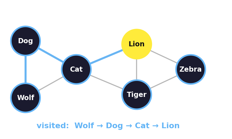
Cat → Lion. The walk crossed the bridge from the “pets” side to the “big cats.”

Cat → Lion。ウォークは橋を渡り「ペット」側から「大型ネコ」へ。

Step 3: Cat -> Lion. The walk crosses the bridge (Cat) between clusters — foreshadows the category-switch in fluency (segment 6).

Take a walk — and keep going歩いてみる — さらに続ける

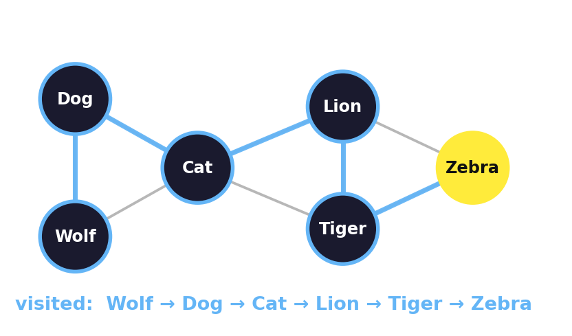
…Lion → Tiger → Zebra. Visited so far: Wolf → Dog → Cat → Lion → Tiger → Zebra.

Run it long enough — which nodes get visited most?

…Lion → Tiger → Zebra。訪問: Wolf → Dog → Cat → Lion → Tiger → Zebra。

十分長く走らせると — どのノードが一番訪れられる?

Final state of the walk build-up. The question on the slide sets up the degree result + poll. ~20s.

The stationary distribution of a walkウォークの定常分布

For an undirected, unweighted network, the long-run visit frequency has a beautifully simple form:

\[\pi_i \;\propto\; \deg(i)\]

where \(\deg(i)\) = the degree of node \(i\) = how many edges touch it, and \(\propto\) means “grows with” — double the edges, roughly double the visits.

More connected → visited more often. No eigen-solve needed for this case — the degree is the answer.

無向・重みなしネットワークでは、長期の訪問頻度は驚くほど単純：

\[\pi_i \;\propto\; \deg(i)\]

ここで \(\deg(i)\) = ノード \(i\) の次数 = 接続するエッジの本数、 \(\propto\) は「に比例して増える」 — エッジが倍なら訪問もおよそ倍。

繋がりが多い → 訪問が多い。 この場合は固有値計算不要 — 次数が答えそのもの。

The clean payoff. Define “degree” inline (first use). Check it against the walk: the highest-degree node was visited most. This is also exactly why PageRank works (Block 8) and why high-degree concepts dominate fluency (Block 6). ~2 min.

Poll — which node wins?ポール — どのノードが勝つ?

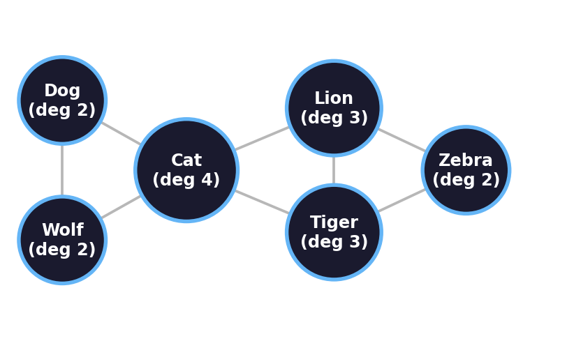
Run a random walk on this network for a long time.

Which node do you visit most often?

• A. Cat
• B. Lion
• C. Wolf
• D. Zebra

このネットワークでランダムウォークを長く走らせる。

最も頻繁に訪れるノードは?

• A. Cat
• B. Lion
• C. Wolf
• D. Zebra

Degree is printed on each node in the figure (but NOT highlighted — no spoiler). Commit before reveal. Cat is the bridge between the two clusters, so it has the most edges (degree 4) — but let students figure that out. ~1 min.

Poll — answerポール — 答え

A. Cat — it has the highest degree.A. Cat — 次数が最も高い。

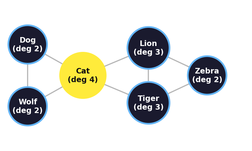
\(\pi_i \propto \deg(i)\), and Cat touches the most edges (degree 4) — it’s the bridge between the two clusters. Long-run behavior is dictated by structure: no extra assumption needed, and no eigen-solve for an undirected graph — the degree is the answer.

Hold onto this: the most-visited concept is the most-connected one. That’s about to explain how people recall.

\(\pi_i \propto \deg(i)\) であり、Cat が最も多くのエッジ（次数4）に接する — 2つのクラスタを繋ぐ橋だから。長期挙動は構造で決まる：追加の仮定も、 無向グラフなら固有値計算も不要 — 次数が答えそのもの。

覚えておいて：最も訪れられる概念は最も繋がった概念。これがこの後、人が どう思い出すかを説明する。

Bridge sentence matters: most-visited = most-connected → this is the engine of the Abbott model after the break. ~1 min.

Where we are現在地

• Welcome + a Markov chain you already knowようこそ + すでに知っているマルコフ連鎖 0:00
• Markov chains: states, transitions, the Markov propertyマルコフ連鎖：状態・遷移・マルコフ性 0:10
• Stationary distribution定常分布 0:25
• Networks: graphs as structureネットワーク：構造としてのグラフ 0:40
• Random walk on a networkネットワーク上のランダムウォーク 0:52
• Break休憩 1:07
• Memory search as a random walk (Abbott 2012)ランダムウォークとしての記憶探索（Abbott 2012） 1:12
• Network properties + PageRank + Week 7 bridgeネットワークの性質 + PageRank + 第7週へ 1:48

Recap ~10s. All the machinery is in place. After the break: the cognitive payoff — this exact model IS a theory of human memory search.

Break休憩

5 minutes

5分

5 min break. After: animal fluency = a random walk on a semantic network (Abbott 2012, the required reading).

Memory search as a random walkランダムウォークとしての記憶探索

Block 6. The required-reading payoff (Abbott, Austerweil & Griffiths 2012). Phenomenon first (the fluency task), then the model. Instructor-led — no presenter this week.

Try it yourselfやってみよう

List as many animals as you can — 60 seconds. Go.

動物をできるだけたくさん挙げて — 60秒。スタート。

Run it live if the room is willing (30-60s), or just have them think it. This is the “verbal/semantic fluency” task (Bousfield & Sedgewick 1944; Troyer et al. 1997). After: ask what ORDER things came out in. Show before tell. ~1.5 min.

What your list looks likeあなたのリストの形

People don’t list animals at random. They come out in bursts by category:

wolf, lion, giraffe, zebra … dog, cat, hamster …

A run of African animals, a pause, a run of pets. Then a switch.

Why this structure? And why those animals, in that order?

人はランダムに動物を挙げない。カテゴリごとのまとまりで出てくる：

オオカミ、ライオン、キリン、シマウマ … イヌ、ネコ、ハムスター …

アフリカの動物の連続、一拍、ペットの連続。そして切り替え。

なぜこの構造? なぜそれらの動物が、その順で?

The empirical phenomenon: clustering + switching. This is what any theory of recall has to explain. Hold the answer one slide. ~1.5 min.

The model: recall is a random walkモデル：想起はランダムウォーク

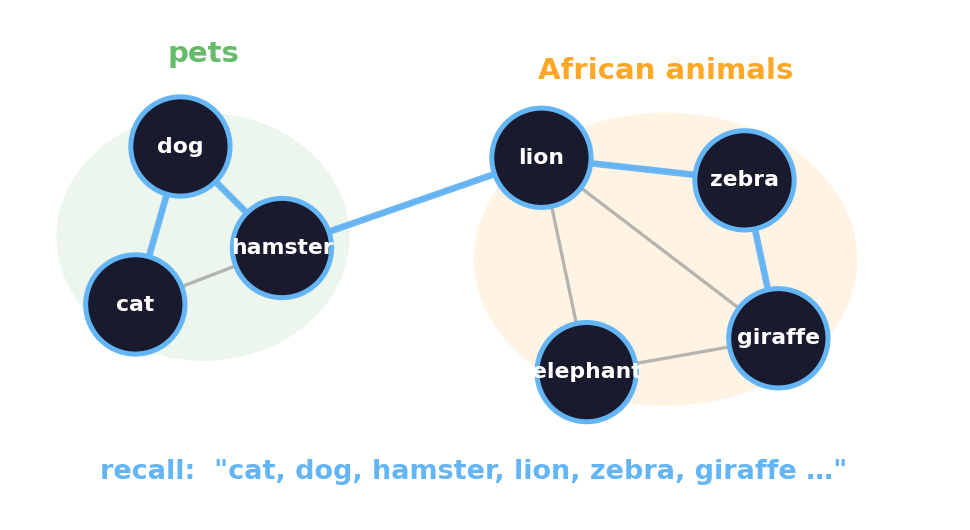
Abbott, Austerweil & Griffiths (2012):

Your semantic memory is a network; recall is a random walk on it. The list you produce is the sequence of nodes the walk visits.

• Clusters = the walk lingering in a densely-connected community
• Switches = the walk crossing a bridge edge to another community

No extra “search strategy” needed — it falls out of the network.

Abbott, Austerweil & Griffiths (2012):

意味記憶はネットワークであり、想起はその上のランダムウォーク。 あなたが出すリストはまさにウォークが訪れるノードの系列。

• まとまり = 密に繋がった共同体に滞在するウォーク
• 切り替え = 別の共同体への橋エッジを渡るウォーク

追加の「探索戦略」は不要 — ネットワークから自然に出る。

THE payoff slide. Everything today converges here: a Markov chain (Block 2) + a network (Block 4) + a random walk (Block 5) = a theory of memory. BUT the raw walk isn’t the fluency list yet — that’s the censoring function, next slide. The required reading. ~2 min.

The catch: the walk ≠ the list落とし穴：ウォーク ≠ リスト

A random walk revisits nodes and wanders through non-animals — but a fluency list has neither. So the walk is not the list directly.

The censoring function (Abbott et al. 2012) is the missing link: you report a word only the first time the walk hits it, and only if it’s an animal. Everything else is censored (hidden).

• \(\tau(k)\) = the first hitting time of the \(k\)-th unique animal
• The gap between first-hits → the inter-item response time (IRT) — what the data actually measures.

ランダムウォークはノードを再訪し、動物以外もさまよう — でも流暢性リストにはどちらもない。だからウォークはそのままではリストではない。

打ち切り関数（Abbott et al. 2012）が欠けていた繋がり：ウォークが初めてその語に到達したときだけ、しかも動物なら報告する。それ以外は打ち切り（隠す）。

• \(\tau(k)\) = \(k\)番目のユニークな動物の初到達時刻
• 初到達の間隔 → 項目間反応時間（IRT） — データが実際に測るもの。

THE crucial mechanism the model needs. Without censoring, the walk is just a node sequence — it isn’t the fluency list and can’t be compared to IRT data. Censoring = report each unique animal only on FIRST hit; everything else (revisits, non-animals) is hidden. tau(k) = first hitting time of the k-th unique animal; IRT = gap between consecutive first-hits (+ word length). This is what links the latent walk to the observed behavior. Worked example next. ~2 min.

Censoring — worked example打ち切り — 具体例

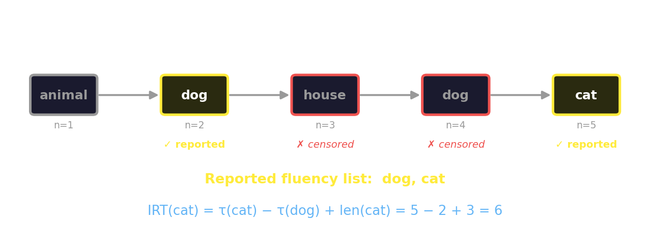
The walk visits animal → dog → house → dog → cat. Reported: dog, cat. house (not an animal) and the second dog (a revisit) are censored. The IRT to “cat” is the step-gap between first-hits, plus the word’s length.

ウォークは animal → dog → house → dog → cat を訪れる。報告：dog, cat。house（動物でない）と2回目のdog（再訪）は打ち切り。「cat」へのIRTは初到達間のステップ差 + 語長。

Walk through it live (the paper’s own example, §4.2). animal(n=1) → dog(n=2, first animal → KEEP) → house(n=3, not an animal → CENSOR) → dog(n=4, revisit → CENSOR) → cat(n=5, first time → KEEP). Reported list: dog, cat. tau(dog)=2, tau(cat)=5. IRT(cat) = 5 − 2 + len(“cat”)=3 → 6. The IRT is read straight off the censored walk — THAT is how the latent process connects to the data. ~2 min.

The signature: slow down, then switch特徴：減速、そして切り替え

The famous optimal-foraging finding (Hills et al. 2012): line up each animal by when it appears relative to a category switch.

• Within a patch, items come faster and faster — until they slow.
• The first word of a new patch is the slowest of all — it’s above your average IRT. That’s the “switch cost.”

Marginal Value Theorem: leave a patch when its return rate drops below your overall average. People look like they’re foraging.

有名な最適採餌の発見（Hills et al. 2012）：各動物をカテゴリ切り替えに対する位置で並べる。

• パッチ内では項目がどんどん速く出てくる — やがて遅くなるまで。
• 新しいパッチの最初の語が最も遅い — 平均IRTを超える。これが「切り替えコスト」。

限界価値定理：パッチの収益率が全体平均を下回ったら離れる。人は採餌しているように見える。

The behavioral phenomenon (Abbott Fig 1a, from Hills et al. 2012). Set it up BEFORE showing the bar chart so students know what to look for: position-1 bar (first word of new patch) is the tallest, above the average line. Hills et al. read this as a deliberate optimal-foraging switch decision (two processes). ~2 min.

…and the random walk reproduces it…そしてランダムウォークが再現する

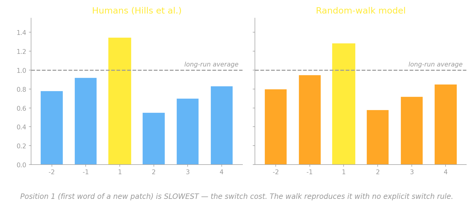
The censored random walk — one process, no switch rule — produces the same curve as humans: position 1 slowest, position 2 fastest. The “decision to switch” was never needed; it falls out of the network’s structure.

打ち切りランダムウォーク — 1つの過程、切り替え規則なし — が人間と同じ曲線を生む：位置1が最も遅く、位置2が最も速い。「切り替えの決定」は不要だった。ネットワークの構造から自然に出る。

THE result (Abbott Fig 3 vs Fig 1a). Left = humans, right = the random-walk model. Same shape: position 1 is the tallest bar (slowest), above the average line. The model has NO switch process — just a censored random walk on the network — yet it reproduces the “switch cost” that was taken as evidence for a deliberate two-process forager. Simpler, unified account. This is the paper’s headline. ~2 min.

Why this is a big claimなぜこれが大きな主張か

The same structure + process split we’ve used since Marr (Week 2):

• Structure — the semantic network (estimated from other behavior, e.g. word-association norms)
• Process — the random walk (a Markov chain — memoryless)
• Behavior — the fluency list (which animals, in which order, with which pauses)

Structure + process jointly predict behavior — and they fit human data well, with no recall-specific machinery bolted on.

Marr 以来（第2週）使ってきた 構造 + 過程 の分け方：

• 構造 — 意味ネットワーク（別の行動、例：語連想規範から推定）
• 過程 — ランダムウォーク（マルコフ連鎖 — 記憶を持たない）
• 行動 — 流暢性リスト（どの動物が、どの順で、どんな間で）

構造 + 過程が行動を共同で予測 — しかも想起専用の仕掛けなしで人間データによく合う。

Tie back to Marr’s levels (Week 2) explicitly — this is the course’s recurring structure/process/behavior frame. The “memoryless” point is the discussion hook: human recall avoids repeats, but a pure random walk doesn’t — is that a problem? (That’s a Slack reflection prompt.) ~2 min.

Discussディスカッション

• The walk is memoryless — but people rarely repeat themselves. Fatal flaw, or fixable?
• The network is estimated from other data. Is that a clean test, or is some explanation smuggled in?
• Does the stationary distribution of your memory mean anything real — salience? accessibility? frequency?

• ウォークは記憶を持たない — でも人はめったに繰り返さない。致命的欠陥? それとも修正可能?
• ネットワークは別データから推定。これはクリーンな検証? それとも説明が紛れ込んでいる?
• あなたの記憶の定常分布は何か現実的なものを意味する? — 顕著性? アクセス可能性? 頻度?

~3 min open discussion (this replaces a student presentation this week). These are the Slack reflection prompts, so students have seen them. Let it breathe. The optional foraging / clinical extensions now come AFTER network properties (post-PageRank), so this discussion flows straight into the network-properties segment. If running short, cut discussion to one question.

Network properties + the road to Week 7ネットワークの性質 + 第7週への道

Block 8. A couple of network terms; ER vs scale-free; PageRank (promised in the Slack thread); the MC->MCMC bridge + close. This segment ALWAYS runs.

A few network termsいくつかのネットワーク用語

• Degree of a node = number of edges touching it. (We used this: \(\pi_i \propto \deg(i)\).)
• Shortest path length (geodesic distance) = fewest edges between two nodes.
• Diameter = the longest shortest-path in the network.
• Degree distribution = the histogram of all nodes’ degrees — it tells you what kind of network you have.

• ノードの次数 = 接続するエッジ数。（\(\pi_i \propto \deg(i)\) で使った。）
• 最短経路長（測地距離） = 2ノード間の最少エッジ数。
• 直径 = ネットワーク内で最長の最短経路。
• 次数分布 = 全ノードの次数のヒストグラム — どの種類のネットワークかを教える。

Brief — these support the figure on the next slide and general literacy. Degree already did real work today. ~1.5 min.

Two kinds of network2種類のネットワーク

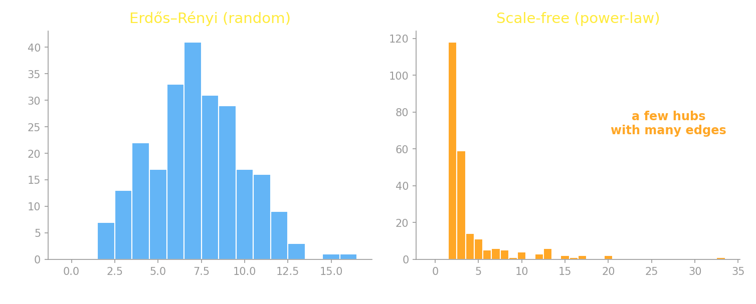
• Random (Erdős–Rényi): Binomial degrees, everyone similar
• Scale-free / power-law: a few high-degree hubs — real semantic, social, and web networks look like this

• ランダム（Erdős–Rényi）： 二項分布の次数、皆似たり寄ったり
• スケールフリー / べき乗則： 少数の高次数ハブ — 実際の意味・社会・ウェブのネットワークはこちら

The two-column figure: random vs scale-free degree distributions. The key contrast: random networks can’t be both sparse AND clustered; real cognitive networks are scale-free, with hubs. Hubs = the high-pi nodes a walk visits most. ~2 min.

Hubs win: PageRankハブが勝つ：PageRank

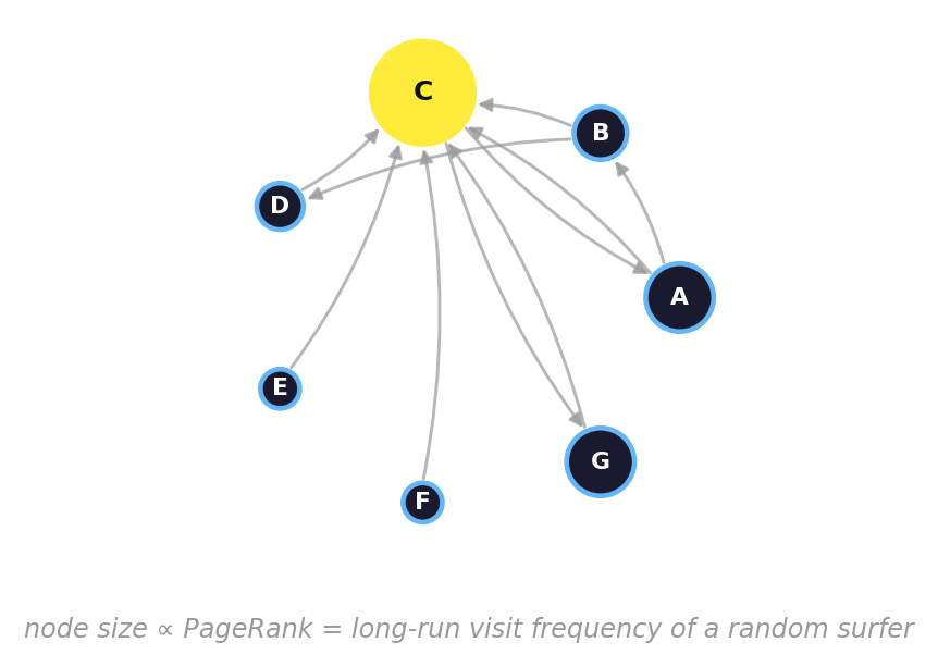
PageRank (the original Google algorithm) ranks pages by the stationary distribution of a random walk over the link graph — exactly the \(\pi\) from this morning, at web scale.

Griffiths, Steyvers & Firl (2007), Google and the mind: PageRank over a semantic network predicts human word-fluency. Same algorithm, same \(\pi\).

PageRank（元祖 Google アルゴリズム）は、リンクグラフ上のランダム ウォークの定常分布でページを順位付け — まさに今朝の \(\pi\) を、ウェブ規模で。

Griffiths, Steyvers & Firl (2007)『Google and the mind』： 意味 ネットワーク上の PageRank が人間の語の流暢性を予測する。同じアルゴリズム、同じ \(\pi\)。

Promised in the Week 6 Slack thread (“the same object behind PageRank, which we’ll see Friday”). The point: pi isn’t an abstraction — it’s a $100B idea AND a model of memory accessibility. A page/concept is important if a random walker visits it often. Makes the whole morning feel real. ~2 min.

Optional: do people actually leave at the optimum?補足：人は本当に最適点で離れる?

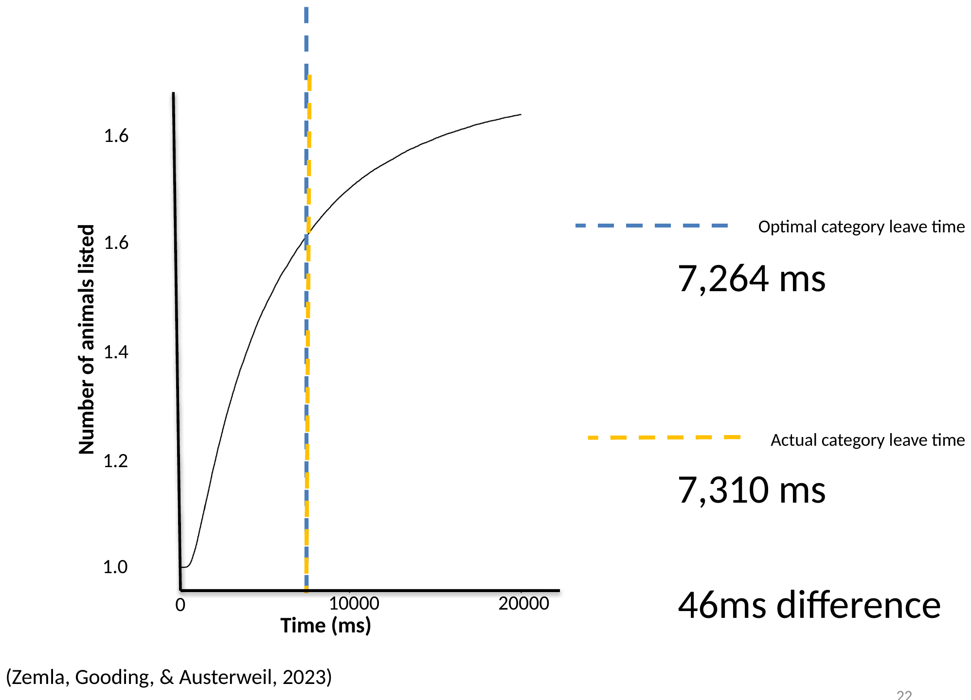
Zemla, Gooding & Austerweil (2023): actual category-leave times track the MVT optimum almost exactly (46 ms apart).

And optimal switching is preserved with age — older adults switch less, but strategically, not from a deficit.

Zemla, Gooding & Austerweil (2023)： 実際のカテゴリ離脱時間は MVT最適値をほぼ正確に追う（46 ms 差）。

そして最適な切り替えは加齢で保たれる — 高齢者はより少なく切り替えるが、 欠陥ではなく戦略的に。

OPTIONAL. Real data. The 46 ms gap is the headline. The age result resolves H1 (“general slowing”) vs H2 (“optimal with fewer resources”) in favor of H2. ~2 min.

Optional: invert the walk → estimate the network補足：ウォークを逆転 → ネットワークを推定

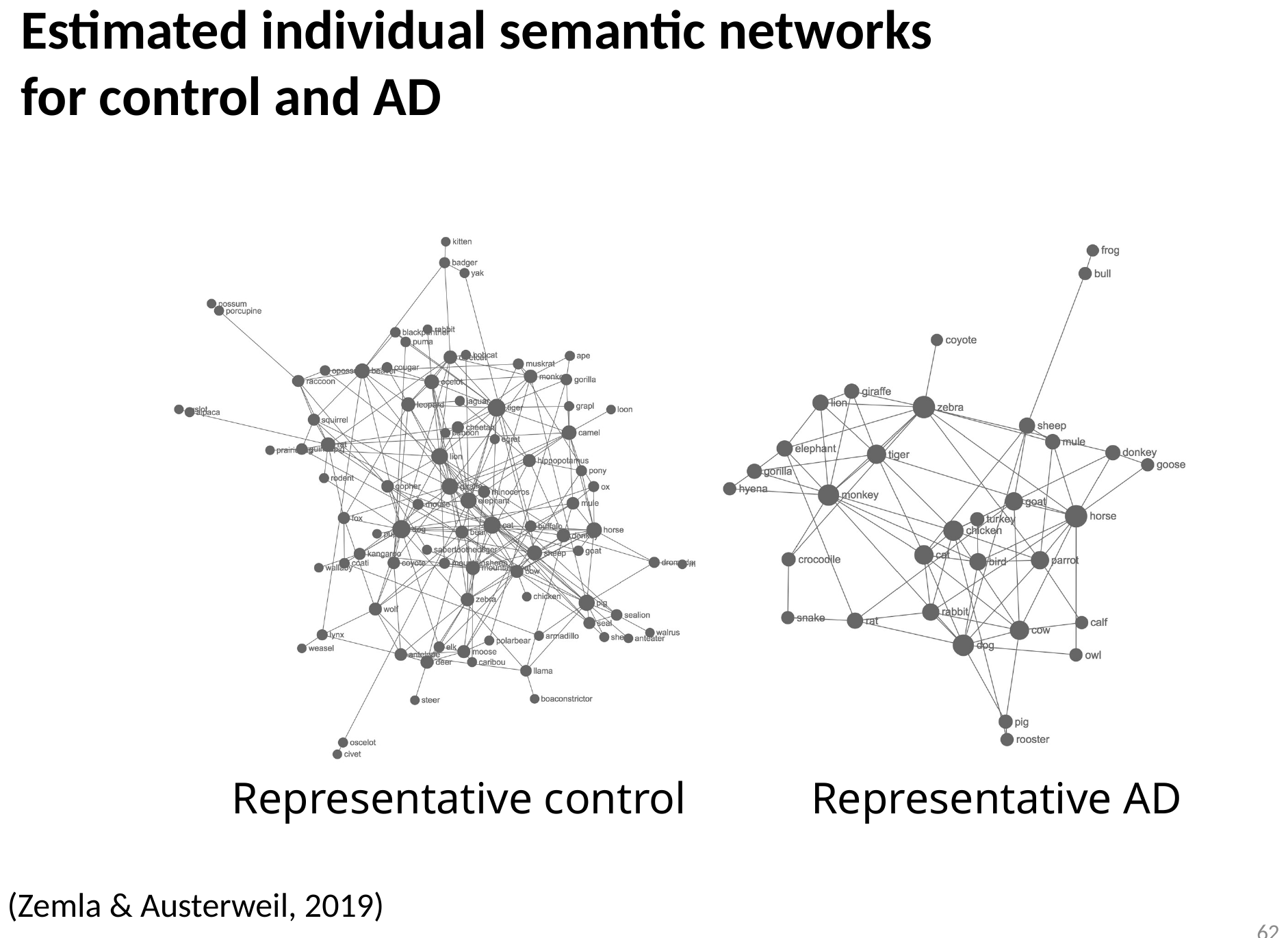
So far: network → walk → fluency list. You can also run it backwards — given fluency lists, infer the most likely network (U-INVITE; Zemla & Austerweil 2018).

That makes the network a measurement instrument: estimate someone’s semantic network from a few fluency lists, then compare groups.

Tool: SNAFU — github.com/AusterweilLab/snafu-py

これまで：ネットワーク → ウォーク → 流暢性リスト。逆向きにも走らせられる — 流暢性リストから最尤ネットワークを推定（U-INVITE；Zemla & Austerweil 2018）。

これでネットワークは測定器になる：数本の流暢性リストから個人の意味ネットワークを推定し、群間比較できる。

ツール：SNAFU — github.com/AusterweilLab/snafu-py

OPTIONAL. The inverse problem (network from behavior). Frame the network as a measurement instrument — that’s what makes the clinical comparison possible (next slide). U-INVITE = the estimation method; SNAFU = the toolkit. ~2 min.

Optional: Alzheimer’s changes the network補足：アルツハイマー病はネットワークを変える

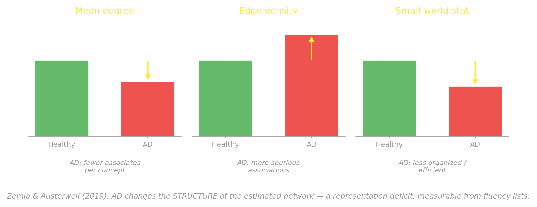
Zemla & Austerweil (2019) estimated networks for 41 AD patients vs. healthy controls. Three structural differences point to an impaired representation — fewer associates per concept, more spurious links, less organized — measured from fluency lists alone. (A separate retrieval deficit — faulty monitoring of what’s already been said — shows up too.)

Zemla & Austerweil (2019) は41名のAD患者と健常対照のネットワークを推定。3つの構造的差異が表現の障害を示す — 概念あたりの連想が少なく、偽の結合が多く、組織化が低い — 流暢性リストだけから測定。（別の検索の障害 — 既出項目の追跡の不全 — も現れる。）

OPTIONAL — the clinical payoff, with the actual Zemla & Austerweil 2019 network-statistic differences. AD networks: smaller MEAN DEGREE (fewer associates), higher EDGE DENSITY (more spurious associations), less SMALL-WORLD-like (less organized). Together = “impaired representation.” A separate retrieval deficit (faulty monitoring) also exists. The headline: a clinical signature read off fluency lists via the network model. This is a presentation candidate this week. ~2 min. End of optional extensions → bridge.

Bridge — we’ve been doing Monte Carlo橋渡し — 私たちはすでにモンテカルロをしていた

Look back at the day:

• Running the chain (Chibany’s bento, the card shuffle) drew samples by comparing a random number to the row of \(P\).
• The stationary distribution we found by running the chain and watching where it settles.

We were estimating a distribution by sampling — that’s Monte Carlo.

今日を振り返ると：

• 連鎖を走らせること（チバニーのお弁当、カードのシャッフル）は、乱数を \(P\) の行と比べてサンプルを引くことだった。
• 定常分布は、連鎖を走らせて落ち着く先を見て求めた。

私たちはサンプリングで分布を推定していた — それがモンテカルロ。

The reframe: we’ve already been using sampling to estimate distributions — running a chain by drawing random numbers IS Monte Carlo. Name it. ~2 min. (The hospital / law-of-large-numbers poll moved to Week 7, where Monte Carlo estimation is the topic.)

Next week — Week 7来週 — 第7週

Monte Carlo — and we flip the problem.

Today the chain came first and we found its stationary distribution. Next week we reverse it: start with a target distribution we want to sample (e.g. a Bayesian posterior), and design a Markov chain whose stationary distribution is that target.

That’s Markov chain Monte Carlo (MCMC) — and it leads to a wild idea: people may sample from their own posteriors (MCMC with People).

Required reading + presenter on the readings page.

モンテカルロ — そして問題を反転する。

今日は連鎖が先にあり、その定常分布を求めた。来週は逆：サンプリング したい目標分布（例：ベイズ事後分布）から始め、その目標を定常分布に持つ マルコフ連鎖を設計する。

それがマルコフ連鎖モンテカルロ（MCMC） — そしてとんでもない 発想へ：人は自分の事後分布からサンプリングしているかもしれない（MCMC with People）。

必須リーディングと発表者はリーディングのページに。

~1.5 min close. The MC->MCMC flip is the whole reason Markov chains came before Monte Carlo in the calendar. Thank the room. Reflections due before next Friday (Abbott or any Week 6 reading). Verify Week 7’s presenter against readings_map.yml before announcing. See you next Friday.