Week 7 — Approximation: Monte Carlo & MCMC第7週 — 近似：モンテカルロとMCMC

Friday, June 12, 20262026年6月12日（金）

Prof. Joseph Austerweilオウステウェイル　ジョセフ教授

Agenda本日の予定

• Admin + What is Monte Carlo? (poll)連絡 + モンテカルロとは?（ポール） 0:00
• Basic Monte Carlo基本のモンテカルロ 0:08
• Importance sampling重点サンプリング 0:23
• Particle filtering粒子フィルタ 0:38
• MCMC: design a chain for a targetMCMC：目標を狙う連鎖を設計 0:48
• Interactive: Gibbs & MHインタラクティブ：ギブズとMH 1:03
• Break休憩 1:15
• Programmable inference (GenJAX)プログラム可能な推論（GenJAX） 1:20
• MCMC with People人を使ったMCMC 1:36
• Sampler for the Kemp modelKemp階層モデルのサンプラー 1:42

~2 min agenda. The spine: we climb a ladder of approximate-inference tools (Monte Carlo -> importance sampling -> particle filter -> MCMC) and then cash it out twice — MCMC with People, and a sampler for the Kemp beta-binomial hierarchy (the model from Week 4). The thread from Week 6: last week we FOUND a chain’s stationary distribution; this week we pick a target and DESIGN a chain to hit it. Throughout, a recurring “in GenJAX” callout maps each method to probabilistic computing. One break. Polls mined from the SP25 Monte Carlo + Markov-chains quizzes.

What is Monte Carlo?モンテカルロとは?

Admin — programming assignment + GenJAX連絡 — プログラミング課題 + GenJAX

Today’s tools are the next programming assignment — a sampler you build yourself.

• We’ll end with the exact recipe for the Kemp hierarchy sampler (the Week 4 model). That recipe is the assignment.
• Walkthrough + stencils: hml.chibatech.dev/assignments.html — GenJAX / Python / R, one-click Colab.
• Reminder: 3 free late days pooled across the four programming assignments.
• Questions? DM me, or the class channel.

今日の道具が次のプログラミング課題 — 自分で組むサンプラー。

• 最後にKemp階層モデルのサンプラー（第4週のモデル）の具体的なレシピを示す。そのレシピが課題そのもの。
• 説明とひな形： hml.chibatech.dev/assignments.html — GenJAX／Python／R、Colabを1クリック。
• 注意：4つのプログラミング課題で共通の無料遅延3日。
• 質問は DM か、クラスチャンネルへ。

~1.5 min. Frame the whole session as building toward the assignment. Don’t re-tour the assignments page. Then the project-proposal slide, then the warm-up poll.

Admin — final project proposal連絡 — 最終プロジェクト提案書

Final project proposal due Sun Jun 28, 8:00 PM — about one page, graded pass/fail.

• Four sections: Background · Question · Method · References (at least 3).
• Three (non-exclusive) categories: experiment · modeling/ML · math/theory — any topic in human and machine learning, not just class material.
• Talk to me about your idea before the deadline — DM or email for 5 minutes.
• Full guidelines: hml.chibatech.dev/project.html

Looking ahead: presentations Fri Jul 17 (final session) · paper due Fri Jul 24.

最終プロジェクトの提案書：6月28日（日）20:00締切 — 約1ページ、合否判定。

• 4つのセクション：背景 · 問い · 方法 · 参考文献（3件以上）。
• 3つの（重複可の）カテゴリ：実験 · モデリング／ML · 数理／理論 — 授業の内容に限らず、人間と機械の学習に関する話題なら何でも。
• 締切前にアイデアを相談してください — DMかメールで5分の面談を。
• 詳細ガイドライン： hml.chibatech.dev/project.html

今後の予定：最終回（7月17日（金））に発表 · 最終レポートは7月24日（金）締切。

~1.5 min. The proposal is the first project deliverable (5%) and the deadline is just over two weeks out — this is the main announcement window. Emphasize the pre-deadline chat: a 5-minute conversation catches too-big/too-small/already- answered questions. Point at the project page for the rubric; don’t tour it. Then straight into the warm-up poll.

Poll — the hospital problemポール — 病院問題

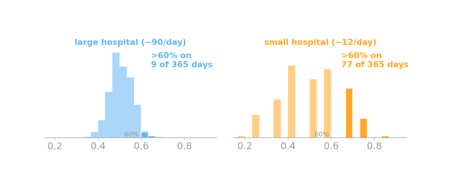
A large hospital and a small hospital each record, over a year, the days where more than 60% of the babies born are boys.

Across the year, which hospital records more such days?

大きい病院と小さい病院が、1年間にわたって、生まれた赤ちゃんの60%超が男の子だった日を記録する。

1年を通して、そういう日が多いのはどちらの病院?

• A. the larger hospital
• B. the smaller hospital
• C. about the same

• A. 大きい病院
• B. 小さい病院
• C. だいたい同じ

Source: SP25 Monte Carlo Estimation quiz, item “Intuition” (Kahneman & Tversky). Run as a FULL poll from scratch this week (the Week-6 commit didn’t happen). Commit before reveal — options appear on the first keypress; have students vote A/B/C, THEN advance to the reveal slide. ~1 min.

Poll — answerポール — 答え

B — the smaller hospital.B — 小さい病院。

Small samples vary more — the law of large numbers. A big sample’s boy-fraction sits tight near 50%; a small one swings wildly, so it crosses 60% on far more days.

小さい標本ほどばらつく — 大数の法則。大きな標本の男の子の割合は50%付近に固まり、小さい標本は大きく振れる。だから60%を超える日がずっと多い。

Reveal sequence: (0) answer + LLN text; (1) the simulation figure fades in — both hospitals centered at 50%, but the SMALL hospital’s daily boy-fraction swings wider, so its >60% tail is 19.4% vs 2.2% for the large one. THEN advance to the next slide for the “that was Monte Carlo” payoff. ~1.5 min.

That was Monte Carloそれがモンテカルロだった

That was Monte Carlo.それがモンテカルロだった。

You judged a probability by reasoning about repeated random samples — and more samples means a tighter answer. Today we make that the central tool.

繰り返しのランダム標本から確率を判断した — 標本が多いほど答えは締まる。今日はそれを中心的な道具にする。

The payoff slide. They’ve just done Monte Carlo reasoning informally (and seen it simulated); today we make it the central tool. ~30s.

Why approximate?なぜ近似する?

Exact Bayesian inference means summing/integrating over all hypotheses — usually intractable.

• Top-down strategy: borrow good samplers from CS/statistics; then ask whether they double as psychological processes.
• When they do, we get rational process models — algorithms that are both good inference and candidate accounts of how the mind computes. (Sanborn et al. 2010; Shi et al. 2010)

厳密なベイズ推論はすべての仮説にわたる和／積分 — たいてい計算不能。

• トップダウン戦略： 計算機科学・統計学から良いサンプラーを借りる。次にそれが心理的過程も兼ねるか問う。
• 兼ねるとき、合理的過程モデルが得られる — 良い推論であり、かつ心の計算の候補説明でもあるアルゴリズム。(Sanborn et al. 2010; Shi et al. 2010)

Marr framing from the SP25 opener. This is the umbrella for BOTH payoffs: MCMC with People (MCMC as a process model) and particle filters (SIS as a process model). ~1.5 min.

Basic Monte Carlo基本のモンテカルロ

The Monte Carlo estimatorモンテカルロ推定量

To estimate an expectation \(\mathbb{E}_{P}[f(x)]\) (the average of \(f\) over draws from \(P\)), draw samples and average:

期待値 \(\mathbb{E}_{P}[f(x)]\)（\(P\) からの引きにわたる \(f\) の平均）を推定するには、標本を引いて平均を取る：

\[\hat\mu_n = \frac{1}{n}\sum_{i=1}^{n} f(x_i), \qquad x_i \sim P(x)\]

\(\hat\mu_n\) = our \(n\)-sample estimate of that mean (the hat means “estimated”).

\(\hat\mu_n\) = その平均の \(n\) 標本推定値（ハットは「推定」の意）。

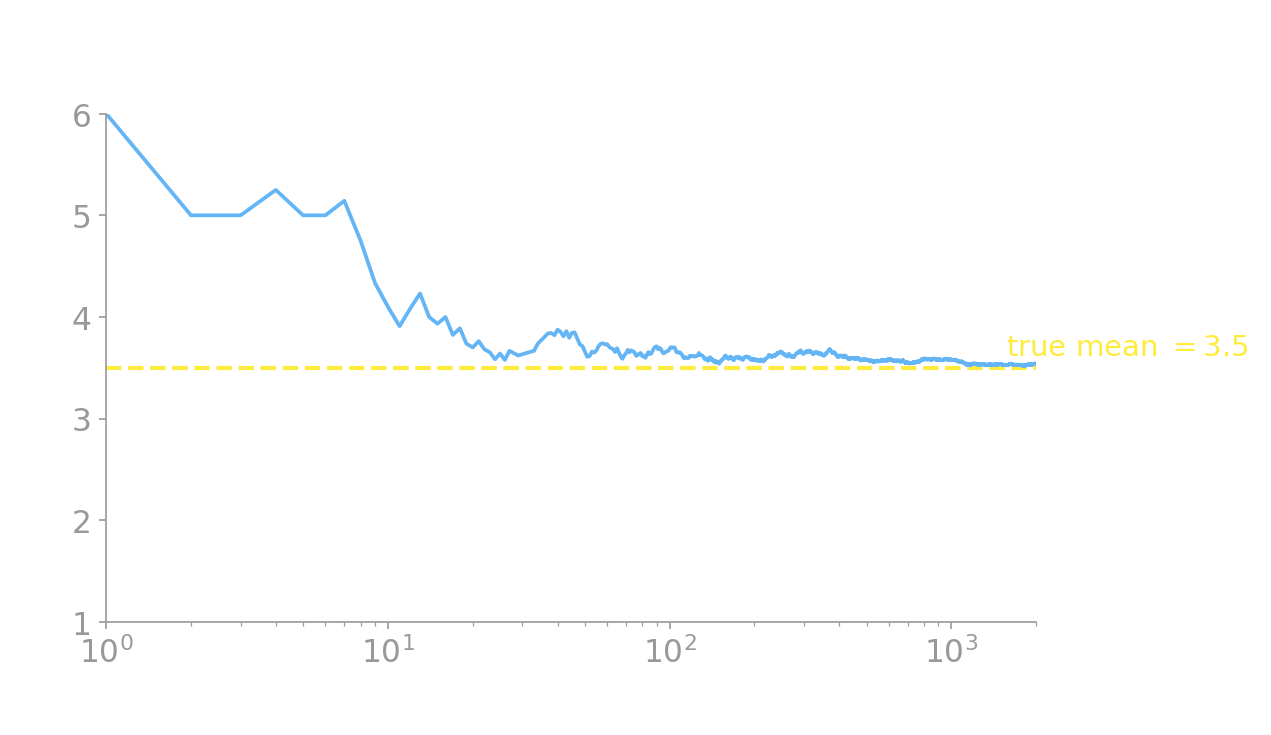
Example — a die roll. The average number of spots is \(\mathbb{E}[x]=3.5\).

Roll it \(n\) times and average. The estimate is noisy for small \(n\) and settles toward 3.5 as \(n\) grows.

例 — サイコロ。 目の平均は \(\mathbb{E}[x]=3.5\)。

\(n\) 回振って平均する。小さい \(n\) では推定はばらつき、\(n\) が増えると 3.5 に落ち着く。

Define the estimator (mu-hat) full-width up top, then the die example as text|figure two-column so the convergence plot is large and legible. The figure IS the LLN from the hospital poll, now visual: small n noisy, large n concentrates. Tie them together explicitly. ~2 min.

Rejection sampling棄却サンプリング

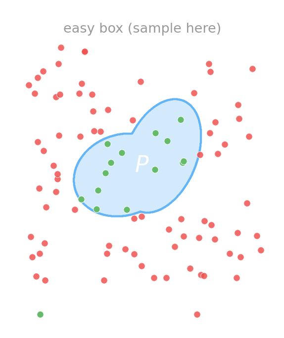
The average above needs samples from \(P\) — but often we can’t draw from \(P\) directly. The simplest fix: rejection sampling.

• Sample from an easy region you can draw from (e.g. a box that contains \(P\)).
• Keep the points that fall under \(P\) (inside the target region); throw away the rest.
• The kept points are distributed exactly as \(P\) — and the fraction kept estimates \(P\)’s area/probability.

Simple and exact, but it wastes samples: if \(P\) fills little of the box, most draws are rejected. The next example makes this concrete.

上の平均には \(P\) からの標本が要る — だが \(P\) から直接引けないことが多い。最も簡単な対処：棄却サンプリング。

• 引ける簡単な領域（例：\(P\) を含む箱）から引く。
• \(P\) の下（目標領域の内側）に落ちた点は残し、それ以外は捨てる。
• 残った点はちょうど \(P\) に従う — そして残った割合が \(P\) の面積／確率を推定する。

単純で厳密だが標本を無駄にする：\(P\) が箱のごく一部しか占めないと大半が棄却される。次の例で具体化する。

NEW full slide (was a half-column shared with inverse-CDF; inverse-CDF removed, and this now comes BEFORE the darts per the reorder — rejection is defined first, then the darts are rejection in action). Define rejection sampling: sample easy, keep-under-P, reject the rest; kept points ~ P; fraction kept = area. Flag the wastefulness -> motivates importance sampling later. ~1.5 min.

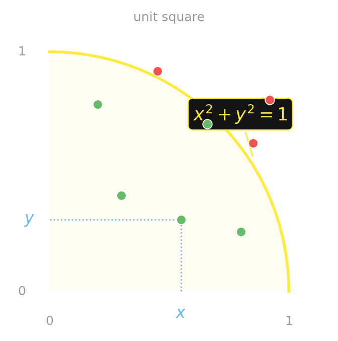
π by throwing darts — rejection in actionダーツで π を求める — 棄却サンプリングの実例

Rejection sampling in action. Throw darts at the unit square (the easy region): draw two uniforms \(x,y \sim \text{Uniform}[0,1]\). Keep a dart when it’s inside the quarter-circle, \(x^2 + y^2 \le 1\); reject the rest.

• Quarter-circle area \(= \pi/4\); square area \(= 1\).
• So the fraction kept \(\approx \pi/4\):

\[\hat\pi = 4\cdot\frac{\#\,\text{inside}}{\#\,\text{total}}\]

This is exactly \(\hat\mu_n\) with \(f(x,y) = \mathbb{1}[x^2+y^2\le 1]\).

\(\mathbb{1}[\cdot]\) = the indicator: 1 when the condition holds, 0 otherwise.

棄却サンプリングの実例。単位正方形（簡単な領域）にダーツを投げる：2つの一様乱数 \(x,y \sim \text{Uniform}[0,1]\) を引く。\(x^2 + y^2 \le 1\) で四分円の内側なら残し、それ以外は棄却。

• 四分円の面積 \(= \pi/4\)、正方形 \(= 1\)。
• だから残った割合 \(\approx \pi/4\)：

\[\hat\pi = 4\cdot\frac{\#\,\text{inside}}{\#\,\text{total}}\]

これはまさに \(f(x,y) = \mathbb{1}[x^2+y^2\le 1]\) の \(\hat\mu_n\)。

\(\mathbb{1}[\cdot]\) = 指示関数：条件が成り立てば1、そうでなければ0。

The canonical two-uniform-draws MC example (Prof. specifically wanted this). The schematic shows the unit square + quarter-circle with x, y, and the arc x^2+y2=1 labeled, plus a few green-inside/red-outside example darts. Define the indicator here — first use. Stress: f is just an indicator, so the average of f IS the probability of landing inside, which IS pi/4. Next slide: watch it converge. ~2 min.

More darts → better estimateダーツが多いほど推定が良くなる

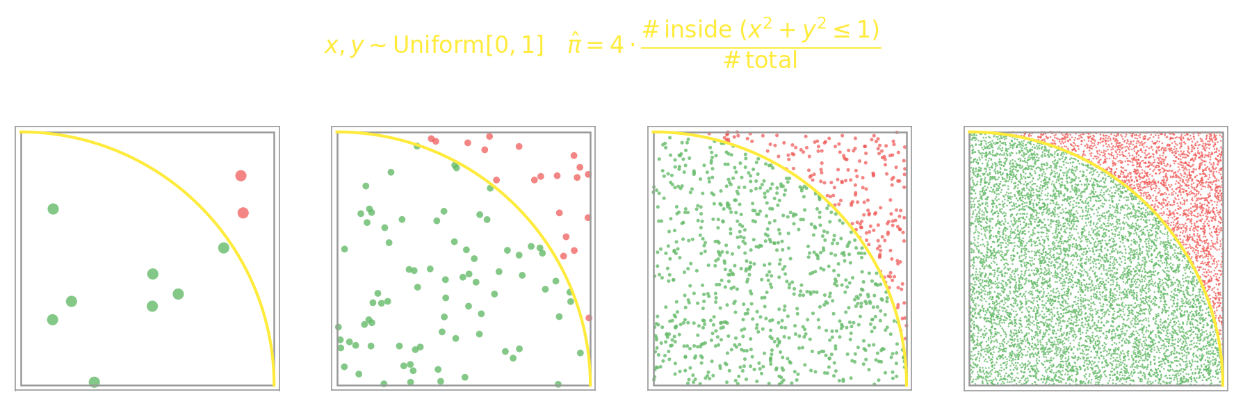
Green = kept (inside), red = rejected (outside). The estimate tightens toward 3.14159… — the same law of large numbers, now in 2-D.

緑=残す（内側）、赤=棄却（外側）。推定値は3.14159…へ締まる — 同じ大数の法則、今度は2次元で。

Build-up: 10 -> 100 -> 1000 -> 10000. At n=10 it’s wildly off; by 10^4 it’s ~3.14. This visually closes the hospital/LLN poll a second time. ~1 min.

What Monte Carlo gives youモンテカルロが保証すること

The estimator \(\hat\mu_n\) is:

• consistent — converges to the truth as data grows: \(\hat\mu_n \to \mathbb{E}[f]\) as \(n\to\infty\).
• unbiased — correct on average even for small \(n\): \(\mathbb{E}[\hat\mu_n] = \mathbb{E}[f]\).
• error shrinks like \(1/\sqrt{n}\) — regardless of dimension (unlike a grid, whose cost explodes as dimensions grow). The estimate’s spread is approximately Gaussian — “asymptotically normal.”

推定量 \(\hat\mu_n\) は：

• 一致性 — データが増えると真値へ収束：\(n\to\infty\) で \(\hat\mu_n \to \mathbb{E}[f]\)。
• 不偏性 — 小さい \(n\) でも平均的には正しい：\(\mathbb{E}[\hat\mu_n] = \mathbb{E}[f]\)。
• 誤差は \(1/\sqrt{n}\) で縮む — 次元によらず （格子は次元とともにコストが爆発するが、MCはしない）。推定値のばらつきはほぼガウス — 「漸近正規」。

But: rejection sampling throws most draws away. Can we instead use every sample, each weighted by how much it tells us about the quantity we’re estimating? → importance sampling. しかし： 棄却サンプリングは大半の引きを捨てる。代わりに、すべての標本を使い、各標本を「推定したい量についてどれだけ情報を持つか」で重み付けできないか? → 重点サンプリング。

One keyword-clause per line. Don’t derive — state. The 1/sqrt(n) “regardless of dimension” is the headline (vs grid methods). The fragment now hinges off rejection’s wastefulness (introduced earlier) into importance sampling. ~1.5 min.

In GenJAX: Monte Carlo is simulate + vmapGenJAXでは：モンテカルロは simulate + vmap

@gen
def dart():
    x = uniform(0.0, 1.0) @ "x"   # throw a dart
    y = uniform(0.0, 1.0) @ "y"
    return (x*x + y*y <= 1.0)     # f = 𝟙[inside]

key  = jax.random.key(0)
keys = jax.random.split(key, 10_000)
sim  = lambda k: dart.simulate(k, ())
traces = jax.vmap(sim)(keys)      # 10k darts
f = traces.get_retval()           # 0/1 per dart
pi_hat = 4.0 * jnp.mean(f)        # π̂ = 4·in/total

• The same darts as before: two uniforms, keep when \(x^2+y^2\le 1\).
• simulate throws one dart (a trace); vmap throws \(n\) in parallel.
• f is the indicator \(\mathbb{1}[\cdot]\); its mean is the fraction inside, so \(\hat\pi = 4\cdot\overline f\).

A probabilistic program’s simulate is the sampler in the estimator.

• さっきと同じダーツ：2つの一様乱数、\(x^2+y^2\le 1\) なら残す。
• simulate は1本のダーツ（トレース）；vmap で \(n\) 本を並列に。
• f こそ指示関数 \(\mathbb{1}[\cdot]\)；その平均が内側の割合なので \(\hat\pi = 4\cdot\overline f\)。

確率的プログラムの simulate こそが推定量の中のサンプラー。

First “in GenJAX” callout, now using the SAME pi-darts example from the rejection slides (Prof. request) so the API maps onto something students just saw. The model draws the two uniforms and returns the indicator f; vmap throws 10k darts; 4*mean(f) is pi_hat. simulate = one dart, vmap = n darts, mean = the estimator. Keep it light. ~1 min. Next slide shows the actual run output (the trace + values).

…and running it…そして実行すると

# peek at the first 5 darts (the trace)
>>> traces.get_choices()["x"][:5]
Array([0.104, 0.091, 0.746, 0.849, 0.610])
>>> traces.get_choices()["y"][:5]
Array([0.228, 0.752, 0.743, 0.928, 0.989])
>>> f[:5]              # 𝟙[x²+y² ≤ 1]
Array([1, 1, 0, 0, 0])

>>> jnp.sum(f)         # darts inside
Array(7859)            # out of 10,000
>>> pi_hat
Array(3.1436, dtype=float32)

• Dart 1 = \((0.10, 0.23)\): \(x^2+y^2 = 0.06 \le 1\) → inside (\(f=1\)).
• Dart 3 = \((0.75, 0.74)\): \(x^2+y^2 = 1.11 > 1\) → outside (\(f=0\)).
• \(7859/10{,}000 = 0.786\) inside, so \(\hat\pi = 4\times 0.786 = 3.14\).

The estimate landed on \(\pi\). Same trace, same indicator, same \(4\cdot\overline f\) as the darts slide — now it’s a probabilistic program.

• ダーツ1 = \((0.10, 0.23)\)：\(x^2+y^2 = 0.06 \le 1\) → 内側（\(f=1\)）。
• ダーツ3 = \((0.75, 0.74)\)：\(x^2+y^2 = 1.11 > 1\) → 外側（\(f=0\)）。
• \(7859/10{,}000 = 0.786\) が内側、よって \(\hat\pi = 4\times 0.786 = 3.14\)。

推定は \(\pi\) に当たった。 ダーツのスライドと同じトレース・同じ指示関数・同じ \(4\cdot\overline f\) — それが確率的プログラムになっただけ。

The SAME pi-darts code as the previous slide, now with the ACTUAL output from a real GenJAX 0.10.3 run (key=0, 10,000 darts, pi_genjax.py). The trace shows the two uniform draws per dart and the indicator f; 7859 darts land inside, so pi_hat = 4*0.7859 = 3.1436. The two worked darts (1 inside, 3 outside) let students verify the indicator by hand. Ties the abstract estimator to a number on the screen AND to the exact darts they saw earlier. ~1.5 min.

Importance sampling重点サンプリング

Sample the wrong distribution — then reweight間違った分布から引いて — 重みで直す

We want \(\mathbb{E}_{P}[f] = \displaystyle\int f(x)\,p(x)\,dx\), but we can’t sample from \(P\).

Idea: sample from an easy distribution \(q\) that we can draw from, and correct for using the wrong one.

求めたいのは \(\mathbb{E}_{P}[f] = \displaystyle\int f(x)\,p(x)\,dx\) だが、\(P\) から標本を引けない。

着想：引ける簡単な分布 \(q\) から引き、間違った分布を使ったことを補正する。

\(p, q\) = the densities of the target \(P\) and the proposal \(q\). Note \(\mathbb{E}_P[f]\) already contains one factor of \(p\) — it’s the \(p(x)\) in the integral.

\(p, q\) = 目標 \(P\) と提案分布 \(q\) の密度。\(\mathbb{E}_P[f]\) は既に \(p\) を1つ含む — 積分の中の \(p(x)\) がそれ。

Setup slide (1/4 of the importance-sampling build-up). The KEY framing that prevents the common error: E_P[f] is the INTEGRAL ∫ f·p dx — it already has one p in it. The trick on the next slide multiplies the integrand by q/q; it does NOT multiply E_P[f] by p (that would double-count p → wrong f·p²/q). ~1 min.

The trick: multiply by \(q/q\)コツ：\(q/q\) を掛ける

Start from the integral, multiply the integrand by \(1 = \dfrac{q(x)}{q(x)}\), and regroup:

積分から始め、被積分関数に \(1 = \dfrac{q(x)}{q(x)}\) を掛けて、まとめ直す：

\[\mathbb{E}_{P}[f] = \int f(x)\,p(x)\,dx = \int f(x)\,p(x)\,\frac{q(x)}{q(x)}\,dx\]

\[= \int \underbrace{f(x)\,\frac{p(x)}{q(x)}}_{\text{new integrand}}\;\underbrace{q(x)\,dx}_{\text{the measure for }\mathbb{E}_q} = \mathbb{E}_{q}\!\left[f(x)\,\frac{p(x)}{q(x)}\right]\]

The leftover \(q(x)\,dx\) is exactly what makes this an expectation under \(q\) — it’s the density we integrate against. This is still an exact identity: no sampling yet. We sample from \(q\) only on the next slide, to estimate this expectation.

残った \(q(x)\,dx\) こそが、これを \(q\) のもとの期待値にする — 積分する密度。これは依然厳密な恒等式：まだサンプリングしていない。\(q\) から標本を引くのは次のスライド、この期待値を推定するためだけ。

The derivation (2/4). The q/q trick, INSIDE the integral. The under-brace makes explicit that one q joins f·p to make the weight and the OTHER q becomes the measure. This is exactly where students (and the prof’s own scratch work) slip: do NOT write E_P[f] = E_P[f·p·q/q] — that inserts a SECOND p. The p is already in the integral; we only insert q/q. ~2 min.

The estimator and the weight推定量と重み

Now it’s an expectation under \(q\) — so estimate it the basic-MC way: draw \(x_i \sim q\) and average.

これは \(q\) のもとの期待値 — だから基本MCのように推定：\(x_i \sim q\) を引いて平均する。

First name the leftover factor — the importance weight \(w(x)\):

まず残った因子に名前を — 重点重み \(w(x)\)：

\[w(x)=\frac{p(x)}{q(x)}\]

\[\mathbb{E}_{P}[f] = \mathbb{E}_{q}\!\left[f(x)\,w(x)\right] \approx \frac{1}{n}\sum_{i=1}^{n} f(x_i)\,w(x_i)\]

Up-weight where \(p > q\), down-weight where \(p < q\). No samples are thrown away — every draw counts, weighted by how useful it is.

\(p > q\) なら重く、\(p < q\) なら軽く。標本は一切捨てない — すべての引きが、有用さに応じた重みで効く。

In practice we usually divide by the sum of the weights instead of \(n\) — the self-normalized estimator: \[\mathbb{E}_{P}[f] \approx \frac{\sum_i f(x_i)\,w(x_i)}{\sum_i w(x_i)}\] Now only ratios of weights appear — which is what lets \(p\) be unnormalized (next slide).

実際には \(n\) ではなく重みの総和で割ることが多い — 自己正規化推定量： \[\mathbb{E}_{P}[f] \approx \frac{\sum_i f(x_i)\,w(x_i)}{\sum_i w(x_i)}\] これで重みの比しか現れない — だから \(p\) を未正規化にできる（次スライド）。

The estimator (3/4). First the plain (1/n) form + the importance weight at first use. Then a fragment introduces the SELF-NORMALIZED form (divide by Σw, not n) — this is what later slides (“p can be unnormalized”, “exemplar models ARE importance samplers”) refer back to, so it must actually appear here. Only ratios of weights survive → p can be unnormalized. ~2 min.

Bonus: \(p\) can be unnormalizedおまけ：\(p\) は未正規化でよい

With self-normalizing (previous slide), only ratios of weights appear, and each weight is itself a ratio \(w = p/q\).

So \(p\) may be unnormalized: if \(p = \tilde p / Z\) for some unknown constant \(Z\), the \(Z\) cancels between numerator and denominator and never matters.

自己正規化（前スライド）により、重みの比しか現れず、各重みも比 \(w = p/q\)。

だから \(p\) は未正規化でよい：\(p = \tilde p / Z\)（\(Z\) は未知定数）なら、\(Z\) は分子と分母で打ち消え、影響しない。

\[\frac{\sum_i f(x_i)\,w_i}{\sum_i w_i} \;=\; \frac{\sum_i f(x_i)\,\dfrac{\tilde p(x_i)}{{\color{red}Z}\,q(x_i)}}{\sum_i \dfrac{\tilde p(x_i)}{{\color{red}Z}\,q(x_i)}} \;=\; \frac{\sum_i f(x_i)\,\dfrac{\tilde p(x_i)}{q(x_i)}}{\sum_i \dfrac{\tilde p(x_i)}{q(x_i)}}\]

The same \({\color{red}Z}\) multiplies every term in both sums, so it factors out and cancels — gone.

This is huge for Bayesian work: a posterior \(p(h\mid d) \propto p(d\mid h)\,p(h)\) is only known up to the constant \(p(d)\) — and importance sampling doesn’t need it.

ベイズでは重要：事後分布 \(p(h\mid d) \propto p(d\mid h)\,p(h)\) は定数 \(p(d)\) を除いてしか分からない — 重点サンプリングはそれを必要としない。

The unnormalized point (4/4), now its own slide instead of a cramped caption. The payoff line connects to Bayesian posteriors (known only up to p(d)) — which is exactly why IS matters for the Kemp model later. ~1 min.

Good \(q\) vs bad \(q\): look at the weights良い \(q\) と悪い \(q\)：重みを見る

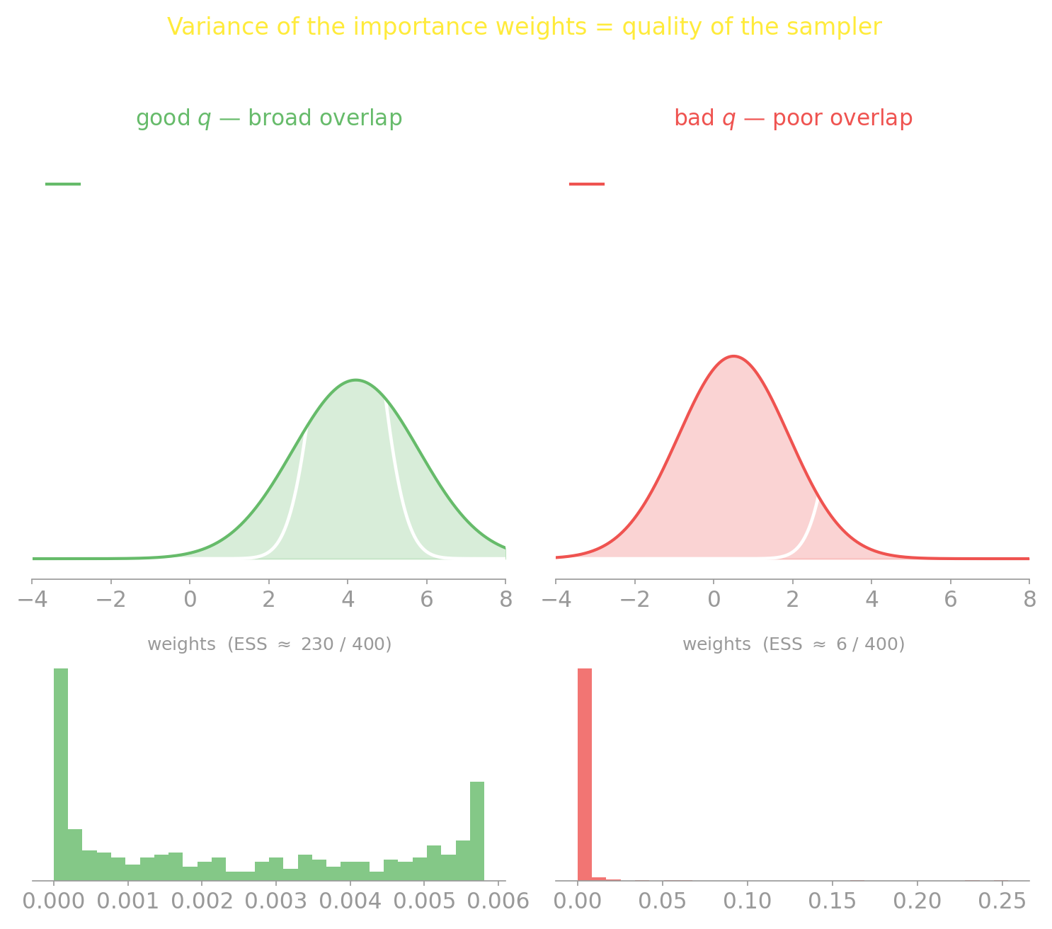
Weight variance = sampler quality. A few huge weights (right) ⇒ effectively a handful of samples (ESS ≈ 6 of 400) ⇒ a noisy estimate. Good \(q\) (left): ESS ≈ 230.

重みのばらつき = サンプラーの質。 少数の巨大な重み（右）⇒ 実質わずかな標本（ESS ≈ 6/400）⇒ ノイズの多い推定。良い \(q\)（左）：ESS ≈ 230。

Good q (broad overlap, even weights, ESS≈230) vs bad q (one weight dominates, ESS≈6). ESS = effective sample size = (Σwᵢ)²/Σwᵢ² — how many independent draws the weighted samples are really worth (out of 400). This diagnostic motivates the “blunt tool” line for Kemp later. Next slide makes ESS a number you compute. ~2 min.

Effective sample size, as a number実効標本サイズ、数値として

Put a number on “how many of my \(T\) weighted samples actually count.” With normalized weights (\(w_t \ge 0\), \(\sum_t w_t = 1\)):

\[N_{\text{eff}} = \frac{1}{\sum_{t=1}^{T} w_t^{\,2}}\]

• All weights equal (\(w_t = 1/T\)) ⇒ \(N_{\text{eff}} = T\). Nothing wasted.
• One weight dominates ⇒ \(N_{\text{eff}} \to 1\). The estimate rests on a single sample.
• It measures how even the weights are — i.e. how well \(q\) covers \(p\) — not how accurate your final estimate is. (Hold onto that distinction; the assignment’s Problem 3 turns on it.)

「\(T\) 個の重み付き標本のうち実際に効くのは何個か」を数値化する。正規化重み（\(w_t \ge 0\)、\(\sum_t w_t = 1\)）で：

\[N_{\text{eff}} = \frac{1}{\sum_{t=1}^{T} w_t^{\,2}}\]

• 重みが全て等しい（\(w_t = 1/T\)）⇒ \(N_{\text{eff}} = T\)。無駄なし。
• 1つの重みが支配⇒ \(N_{\text{eff}} \to 1\)。推定が1標本に依存。
• これは重みの均等さ（= \(q\) が \(p\) をどれだけ覆うか）を測る — 最終推定の正確さではない。（この区別を覚えておく；課題の問題3の核心。）

NEW slide (added for the assignment: Problem 3 needs N_eff as a computable quantity, not just the dim caption on the previous figure). The formula, the two limits (uniform -> T, peaked -> 1), and the key warning that ESS measures weight- evenness NOT estimator accuracy – which is exactly the Problem 3(b) puzzle (plain MC gets N_eff = T yet IS is the better estimator). Don’t belabor; the PDF carries the full puzzle. ~1.5 min.

The simplest importance sampler最も簡単な重点サンプラー

For a posterior \(P(h\mid d)\), use the prior as the proposal: \(q = P(h)\). Then the weights are just the likelihood:

事後分布 \(P(h\mid d)\) には、事前分布を提案に使う：\(q = P(h)\)。すると重みは尤度そのもの：

\[w(h) = \frac{P(h\mid d)}{P(h)} = \frac{P(d\mid h)\,P(h)}{P(d)\,P(h)} = \frac{P(d\mid h)}{P(d)} \;\propto\; P(d\mid h)\]

Sample from the prior, weight by the likelihood. That’s the whole recipe.

We don’t know \(P(d)\), so divide by the sum of the weights instead of \(1/n\) — this is self-normalized importance sampling: \(\;\mathbb{E}[f]\approx \sum_i f(h_i)w_i / \sum_i w_i\).

事前から引き、尤度で重み付け。 これがレシピのすべて。

\(P(d)\) は未知なので、\(1/n\) ではなく重みの総和で割る — これが自己正規化重点サンプリング：\(\;\mathbb{E}[f]\approx \sum_i f(h_i)w_i / \sum_i w_i\)。

Likelihood weighting. The P(d) cancels into a normalizing constant -> self- normalized IS. This is the pattern GenJAX’s .importance gives you for free (next-but-one slide). ~1.5 min.

Exemplar models are importance samplers事例モデルは重点サンプラーである

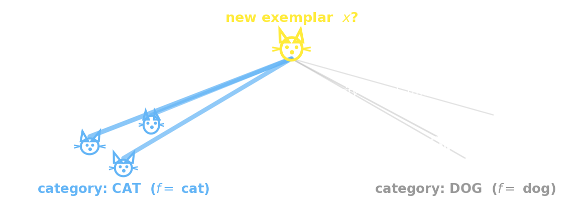
A cognitive aside that recurs all term. Exemplar models (Nosofsky 1986) answer with a similarity-weighted vote over stored examples (\(x_i\)):

学期を通じて再登場する認知の余談。事例モデル（Nosofsky 1986）は、記憶した例（\(x_i\)）にわたる類似度重み付き投票で答える：

\[\text{response}(x) = \frac{\sum_i s(x, x_i)\,f(x_i)}{\sum_i s(x, x_i)}\]

\(s(x, x_i)\) = similarity between the query \(x\) and stored example \(x_i\) (the weight); \(f(x_i)\) = the label/output stored with example \(i\).

\(s(x, x_i)\) = クエリ \(x\) と記憶例 \(x_i\) の類似度（重み）；\(f(x_i)\) = 例 \(i\) に保存されたラベル／出力。

This is exactly the self-normalized importance sampler from earlier (\(\sum_i w\,f / \sum_i w\)) — the stored exemplars are the samples, and similarity \(s\) plays the role of the weight \(w\).

これは先ほどの自己正規化重点サンプラーそのもの（\(\sum_i w\,f / \sum_i w\)）— 記憶した事例が標本、類似度 \(s\) が重み \(w\) の役割。

The course through-line: a famous psychological model turns out to be an inference algorithm. Optional/compressible if behind. ~1.5 min.

In GenJAX: importance sampling for freeGenJAXでは：重点サンプリングが無料

# the model's PRIOR is the default proposal
trace, log_weight = model.importance(
    key, constraint, args)

# score a custom proposal yourself
log_p, retval = model.assess(choices, args)

# K particles (sequential Monte Carlo)
alg = smc.ImportanceK(
    Target(model, args, constraint),
    k_particles=100)

• importance returns a sample and its log_weight — “sample from prior, weight by likelihood” in one call.
• assess scores choices under the model — the primitive you’ll reuse for MCMC.

• importance は標本とその log_weight を返す — 「事前から引き、尤度で重み付け」を1呼び出しで。
• assess はモデル下で選択を採点 — MCMCで再利用する基本演算。

The key map: .importance IS likelihood weighting. The prior is the default proposal, so you get the previous slide’s recipe for one call. Flag assess now — it’s the scoring primitive that MCMC needs. ~1.5 min.

…importance sampling, run…重点サンプリングを実行

# coin with unknown bias; observe heads
@gen
def coin():
    theta = beta(2.0, 2.0) @ "theta"
    y = flip(theta) @ "y"
    return theta

obs = C["y"].set(True)          # condition: heads
def one(k):
    tr, logw = coin.importance(k, obs, ())
    return tr.get_retval(), logw
thetas, logws = jax.vmap(one)(
    jax.random.split(key, 5000))
# self-normalize: weight by the likelihood
w = jnp.exp(logws); w = w / w.sum()
post_mean = jnp.sum(w * thetas)

>>> logws[0]    # = log p(heads|θ)
Array(-0.216, dtype=float32)

>>> thetas[:3]  # prior draws of θ
Array([0.806, 0.485, 0.455],
      dtype=float32)

>>> post_mean   # E[θ | heads]
Array(0.605, dtype=float32)

# true posterior Beta(3,2)
#   mean = 0.600  ✓

Sampled \(\theta\) from the prior, weighted each by the likelihood of heads — the estimate \(0.605\) matches the exact posterior mean \(0.600\).

\(\theta\) を事前から引き、表の尤度で重み付け — 推定 \(0.605\) は厳密な事後平均 \(0.600\) に一致。

The importance-sampling output slide, with ACTUAL output from a real GenJAX 0.10.3 run. A coin: theta ~ Beta(2,2), observe y=heads. coin.importance returns (trace, log_weight) where log_weight = log p(heads|theta) = the likelihood. Self-normalize (weight by exp(logw), divide by the sum) → E[theta|heads] = 0.605, matching the exact Beta(3,2) posterior mean 0.600. This is “sample from prior, weight by likelihood” made concrete, AND a beta-bernoulli preview of the Kemp model. ~1.5 min.

Poll — when the prior is a bad proposalポール — 事前が悪い提案のとき

You importance-sample a posterior using the prior as \(q\). The prior and posterior barely overlap. What happens to your estimate?

事前を \(q\) として事後分布を重点サンプリングする。事前と事後がほとんど重ならない。推定はどうなる?

• A. a few samples get huge weights — the estimate is noisy
• B. all weights are equal — the estimate is exact
• C. every sample is rejected

• A. 少数の標本が巨大な重みを持つ — 推定はノイズだらけ
• B. すべての重みが等しい — 推定は厳密
• C. すべての標本が棄却される

A — weight variance blows up. This is exactly why the textbook’s importance sampling for the Kemp hyperparameters was a “blunt tool.” We fix it with MCMC. A — 重みのばらつきが爆発。これがまさに、教科書のKemp超パラメータの重点サンプリングが「鈍い道具」だった理由。MCMCで直す。

Sourced fresh (IS overlap intuition). Optional — cut first if behind. It sets up the “blunt tool” callback for Block 9. Note A and C are both tempting; C is the rejection-sampling answer, A is the IS answer. ~1 min.

Particle filtering粒子フィルタ

Data arriving over time時間とともに届くデータ

When data come one at a time, recomputing \(P(h\mid d_1,\dots,d_n)\) from scratch each step is wasteful. Exploit a simple fact:

データが1つずつ届くとき、毎回 \(P(h\mid d_1,\dots,d_n)\) をゼロから計算し直すのは無駄。簡単な事実を使う：

\[P(h\mid d_1,\dots,d_n) \;\propto\; P(d_n\mid h)\;\underbrace{P(h\mid d_1,\dots,d_{n-1})}_{\text{yesterday's posterior}}\]

Yesterday’s posterior is today’s prior. Repeated importance sampling over a growing dataset = a particle filter (a.k.a. sequential Monte Carlo).

昨日の事後分布が今日の事前分布。 増えていくデータに対する繰り返しの重点サンプリング = 粒子フィルタ（逐次モンテカルロ）。

SIS. The recursion IS Bayes applied incrementally. Names: particle filter, SMC, bootstrap filter, condensation, survival of the fittest. ~2 min.

The particle filter粒子フィルタの仕組み

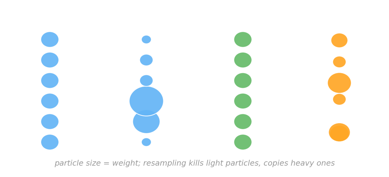
Init \(M\) particles from the prior. Per datum: weight by \(P(d_n\mid h)\), normalize, and resample if the weights degenerate (kill light particles, copy heavy ones).

\(M\) 個の粒子を事前から初期化。各データで：\(P(d_n\mid h)\) で重み付け、正規化、重みが偏れば再サンプリング（軽い粒子を捨て、重い粒子を複製）。

Walk the schematic left to right. Resampling is the trick that stops all the weight piling onto one particle. ~2 min.

A worked example: tracking a moving object実例：動く物体を追跡する

A robot slides along a line; we want its position over time. We carry 5 particles — guesses for where it is. Tracking over time needs two modeling assumptions — the same two any state-space model makes:

ロボットが直線上を滑る。各時刻での位置を知りたい。5粒子（位置の推測）を運ぶ。時間追跡には、状態空間モデルが常に置く2つのモデル仮定が必要：

• Observation model \(P(z \mid x)\) — how a state produces a sensor reading. Here: \(z \sim \mathcal{N}(x, \sigma^2)\) (noisy sensor). Gives the weight \(w_i \propto P(z \mid x_i)\).
• Motion model \(P(x_{t} \mid x_{t-1})\) — how the state evolves between ticks. Here we assume the robot drifts \(+1\) with a little noise. Used to propagate.

Both are your modeling choices, not facts. If the thing doesn’t move, the motion model is just “stay put” (\(x_t = x_{t-1}\)) — particle filtering doesn’t require dynamics, only that you state some transition.

• 観測モデル \(P(z \mid x)\) — 状態がどうセンサ値を生むか。ここでは \(z \sim \mathcal{N}(x, \sigma^2)\)（ノイズ付きセンサ）。重み \(w_i \propto P(z \mid x_i)\) を与える。
• 運動モデル \(P(x_{t} \mid x_{t-1})\) — 状態が刻みの間にどう変化するか。ここではロボットが少しのノイズ付きで \(+1\) ドリフトすると仮定。伝播に使う。

どちらもあなたのモデル選択であって事実ではない。対象が動かないなら、運動モデルは単に「その場に留まる」（\(x_t = x_{t-1}\)）— 粒子フィルタは動力学を要求しない。何らかの遷移を述べればよいだけ。

Set up the 1-D tracking problem before the three step slides. CRITICAL framing (Prof. note): a particle filter is inference in a STATE-SPACE model, which has TWO assumed pieces — the observation model (gives weights) and the motion/ transition model (gives propagation). Both are modeling choices, NOT given. The “+1 drift” in Step 3 is an ASSUMPTION, introduced here so it isn’t a surprise. Defuse the misconception that PF needs dynamics: a static state just uses the identity transition (x_t = x_{t-1}) — PF still works, you just don’t move the particles. The state (x_i), observation (z), weight (w_i) symbols recur on every step figure. ~2 min.

Step 1 — weight by the observationステップ1 — 観測で重み付け

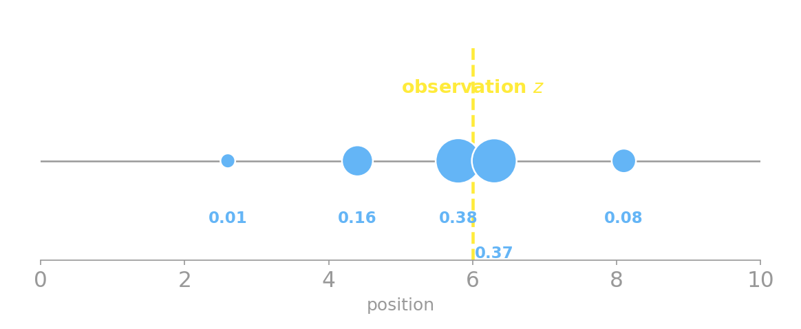
Each particle gets a weight \(w_i \propto P(z \mid x_i)\) — bigger dots are heavier. The two particles flanking the observation carry almost all the weight; the far ones are nearly zero.

各粒子に重み \(w_i \propto P(z \mid x_i)\) — 大きい点ほど重い。観測の両隣の2粒子がほぼ全重みを持ち、遠い粒子はほぼゼロ。

The weights ARE importance weights — this is sequential importance sampling. Particles near z (the yellow line) explain the data well. ~1 min.

Step 2 — resampleステップ2 — 再サンプリング

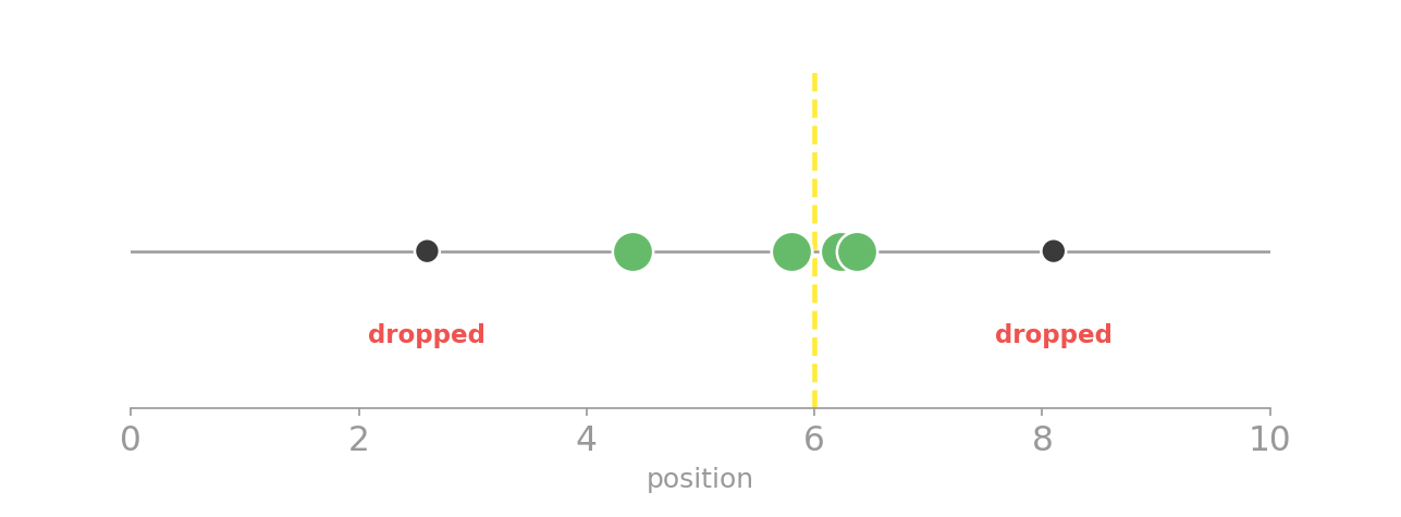
Draw 5 new particles with replacement, each chosen with probability \(\propto w_i\). Heavy particles get copied (sometimes twice); the two far-from-\(z\) particles are dropped. Same particle count, mass now concentrated where the data points.

確率 \(\propto w_i\) で5個の新しい粒子を復元抽出。重い粒子は複製され（時に2回）、\(z\) から遠い2粒子は捨てられる。粒子数は同じだが、質量はデータの指す場所に集中。

Resampling kills the degeneracy: without it, one particle would eventually hog all the weight. After resampling the weights reset to uniform. ~1 min.

Step 3 — propagateステップ3 — 伝播

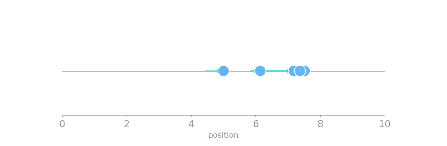
Push every particle forward through the assumed motion model \(P(x_t \mid x_{t-1})\) from the setup (here: drift \(+1\), plus a little noise). The cloud is now this tick’s prior — ready to be weighted by the next observation. Loop back to Step 1. (Static target? This step is just \(x_t = x_{t-1}\) — the particles stay put.)

各粒子を設定で仮定した運動モデル \(P(x_t \mid x_{t-1})\) で前進（ここでは：ドリフト \(+1\) と少しのノイズ）。この雲が今刻みの事前分布 — 次の観測で重み付けする準備完了。ステップ1へ戻る。（対象が静止？ この手順は単に \(x_t = x_{t-1}\) — 粒子はその場に留まる。）

Propagate = apply the transition. This closes the loop: propagated cloud is the prior for the next weight step. weight->resample->propagate, repeat. ~1 min.

The particle filter in GenJAXGenJAXでの粒子フィルタ

@gen
def step(x_prev):
    x = normal(x_prev + 1.0, 0.5) @ "x"  # propagate
    z = normal(x, 1.2) @ "z"             # observe
    return x

def filter(key, observations, xs):
    for z in observations:
        k1, k2, key = jax.random.split(key, 3)
        # weight: importance over all particles at once
        keys = jax.random.split(k1, len(xs))
        tr, log_w = jax.vmap(lambda k, xp:
            step.importance(k, C["z"].set(z), (xp,))
        )(keys, xs)
        # resample ∝ weight
        idx = jax.random.categorical(k2, log_w,
                                     shape=xs.shape)
        xs = tr.get_choices()["x"][idx]
    return xs

• The same three steps: importance = weight, categorical = resample, the next loop’s simulate inside step = propagate.
• importance returns each particle and its log_weight — no hand-derived likelihood.
• vmap runs all particles in parallel on one device.

• 同じ3ステップ：importance = 重み付け、categorical = 再サンプリング、次ループの step 内 simulate = 伝播。
• importance は各粒子とその log_weight を返す — 尤度を手で導出しない。
• vmap で全粒子を1デバイス上で並列実行。

The bootstrap filter, hand-rolled — 0.10.3 has no high-level chain(), so we write the loop. The point: importance/categorical/simulate ARE the three algorithm steps. Upstream v1.0.10 packages this as smc helpers. ~2 min.

…the filter, run…フィルタを実行

# object drifts +1 per tick from 1
true  = [1, 2, 3, 4, 5]
# noisy sensor readings
obs   = [1.3, 1.8, 3.4, 3.9, 5.2]

ests = []
xs = init_particles(key, M=1000)
for z, x in run(key, obs):
    ests.append(float(jnp.mean(xs)))

true  : [1.0, 2.0, 3.0, 4.0, 5.0]
obs   : [1.3, 1.8, 3.4, 3.9, 5.2]
PF est: [1.1, 1.96, 3.07, 4.01, 5.08]

• The filter’s mean tracks the true position [1, 2, 3, 4, 5] — even though it only ever sees the noisy observations.
• It smooths: the estimate \(1.96\) at tick 2 is pulled back toward the track from the noisy \(1.8\), because the motion model says “you should be near 2.”
• 1000 particles, real GenJAX 0.10.3 output.

• フィルタの平均は真の位置 [1, 2, 3, 4, 5] を追う — ノイズの多い観測しか見ていないのに。
• 平滑化する：刻み2での推定 \(1.96\) は、運動モデルが「2付近のはず」と言うので、ノイズの多い \(1.8\) から軌道側へ引き戻される。
• 1000粒子、実際の GenJAX 0.10.3 出力。

Real run (pf_genjax.py). The headline: PF est tracks the true track, smoothing the noisy obs — motion model + observations combined. This is exactly the worked example, now in code with 1000 particles. ~1.5 min.

Particle filters as process models過程モデルとしての粒子フィルタ

Why this, of all approximations? A particle filter is a probabilistic approximation that builds incrementally — yesterday’s posterior is today’s prior. But “incremental + probabilistic” alone isn’t special (exact recursive Bayes is too). What makes it a cognitive model is the shape of its approximation: it holds a small, fixed number of concrete hypotheses (\(M\) particles), updated by stochastic resampling.

That specific form predicts the ways people deviate from full Bayes:

• limited memory — only \(M\) hypotheses carried forward (people track a handful, not a full distribution; \(M\) is a fittable “how-approximate” knob).
• order effects — early data decide which particles survive (Kruschke 2006); a parametric incremental filter wouldn’t predict this.
• variability — resampling is random, so two people (two runs) can land on different beliefs from the same data.

Applied to feature learning (Austerweil & Griffiths 2013), categorization (Sanborn et al. 2006), associative learning, changepoint detection, sentence processing. In GenJAX: smc.* chained over the observations.

なぜ数ある近似の中でこれか？ 粒子フィルタは逐次的に構築する確率的近似 — 昨日の事後分布が今日の事前分布。だが「逐次的＋確率的」だけでは特別でない（厳密な逐次ベイズもそう）。認知モデルにするのは近似の形：少数で固定個数の具体的仮説（\(M\) 粒子）を、確率的な再サンプリングで更新する点。

その形こそが、人が完全ベイズから逸脱する仕方を予測する：

• 限られた記憶 — 前へ運ぶ仮説は \(M\) 個だけ（人は完全な分布でなく少数を追う；\(M\) は「どれだけ近似か」の調整つまみ）。
• 順序効果 — 早いデータがどの粒子が生き残るかを決める（Kruschke 2006）；パラメトリックな逐次フィルタはこれを予測しない。
• ばらつき — 再サンプリングは確率的なので、同じデータでも2人（2回の実行）が異なる信念に至りうる。

特徴学習（Austerweil & Griffiths 2013）、カテゴリ化（Sanborn et al. 2006）、連合学習、変化点検出、文処理に応用。GenJAXでは： 観測にわたって連鎖させた smc.*。

Answers the Prof’s question “why PF, not just any incremental approximation?” The honest argument: incremental+probabilistic is necessary but NOT sufficient (exact recursive Bayes / Kalman is also incremental + probabilistic and predicts NO human deviations). What singles out the PF is the FORM of its approximation — a finite sample of discrete hypotheses (M particles) updated by stochastic resampling. That specific form is what reproduces the documented human signatures: few hypotheses (Vul et al. 2014 “one and done”), order/primacy effects, and run-to-run variability. Contrast: a parametric incremental filter (assumed-density / variational) smooths the posterior into a Gaussian and predicts none of these. So M is a fittable approximation-budget knob a normative model doesn’t have. Refs: Sanborn, Griffiths & Navarro 2010; Vul, Goodman, Griffiths & Tenenbaum 2014; Abbott & Griffiths. ~2 min.

MCMC: design a chain to hit a targetMCMC：目標を狙う連鎖を設計

Running Week 6 backwards第6週を逆向きに走らせる

Last week you found a chain’s stationary distribution \(\pi\) by running it.

\(\pi\) is stationary when \(\pi P = \pi\) — one more step doesn’t change it.

This week we reverse it: start with a target \(P(x)\) we want (a posterior), and design a Markov chain whose stationary distribution is \(P(x)\). That’s Markov chain Monte Carlo (MCMC).

先週は、連鎖を走らせて定常分布 \(\pi\) を見つけた。

\(\pi\) は \(\pi P = \pi\) のとき定常 — もう1ステップ進めても変わらない。

今週は逆向き：欲しい目標 \(P(x)\)（事後分布）から始め、その定常分布が \(P(x)\) になるマルコフ連鎖を設計する。これが マルコフ連鎖モンテカルロ（MCMC）。

Two schemes: Metropolis–Hastings and Gibbs. 2つの方式：メトロポリス・ヘイスティングスとギブズ。

The named callback to Week 6 — one line, don’t re-derive pi. The “reverse the arrow” framing is the conceptual core of the week. ~1.5 min.

Metropolis–Hastingsメトロポリス・ヘイスティングス

(Metropolis et al. 1953; Hastings 1970)   \(x^{(t)}\) = the state at iteration \(t\).

• Step 0. Start anywhere: \(x^{(0)}\).
• Step 1. Propose a move \(x' \sim Q(x'\mid x^{(t)})\). \(Q\) = the proposal — usually a Gaussian step \(Q=\mathcal{N}(x^{(t)}, \sigma^2)\), width \(\sigma\). (\(\mathcal{N}(\mu,\sigma^2)\) = Normal, mean \(\mu\), variance \(\sigma^2\).)
• Step 2. Accept with probability \(A = \min\!\left(1,\, \dfrac{P(x')}{P(x^{(t)})}\right)\) (symmetric-proposal form). Otherwise stay.

(Metropolis et al. 1953; Hastings 1970)   \(x^{(t)}\) = 反復 \(t\) での状態。

• 手順0. どこからでも開始：\(x^{(0)}\)。
• 手順1. 移動を提案：\(x' \sim Q(x'\mid x^{(t)})\)。\(Q\) = 提案分布 — ふつうガウスのステップ \(Q=\mathcal{N}(x^{(t)}, \sigma^2)\)、幅 \(\sigma\)。（\(\mathcal{N}(\mu,\sigma^2)\) = 正規分布、平均 \(\mu\)・分散 \(\sigma^2\)。）
• 手順2. 確率 \(A = \min\!\left(1,\, \dfrac{P(x')}{P(x^{(t)})}\right)\) で受理（対称提案の形）。さもなくば留まる。

Intuition: a move uphill (toward higher \(P\)) is always accepted; a move downhill is accepted sometimes, in proportion to how far down it goes. That’s what lets the chain explore yet still favor high-probability regions.

直観：上り（\(P\) が高い方）への移動は必ず受理。下りはときどき受理 — どれだけ下るかに比例して。これが、連鎖が探索しつつも高確率領域を好む仕組み。

A Gaussian step is symmetric (\(Q(x'\mid x)=Q(x\mid x')\)), so the \(Q\) terms cancel and only \(P(x')/P(x)\) is left — that’s the Metropolis special case. (Full Hastings keeps a \(Q(x\mid x')/Q(x'\mid x)\) factor for asymmetric proposals.) And only the ratio of \(P\) matters, so the normalizing constant cancels — you never need \(P(d)\). ガウスのステップは対称（\(Q(x'\mid x)=Q(x\mid x')\)）なので \(Q\) が打ち消え、\(P(x')/P(x)\) だけが残る — これがメトロポリスの特別な場合。（一般のヘイスティングスは非対称提案のため \(Q(x\mid x')/Q(x'\mid x)\) を残す。）さらに \(P\) の比だけが効くので正規化定数も打ち消え、\(P(d)\) は要らない。

Define proposal Q (now concrete: Gaussian width sigma), acceptance ratio A, and the iteration superscript x^(t) at first use. Two cancellations: (1) symmetric Q cancels -> Metropolis special case (answers “where did the Hastings term go?”); (2) normalizer cancels -> why MCMC beats exact inference. The sigma here is the demo’s slider. ~2 min.

MH, step by step (1/3)MH、一歩ずつ (1/3)

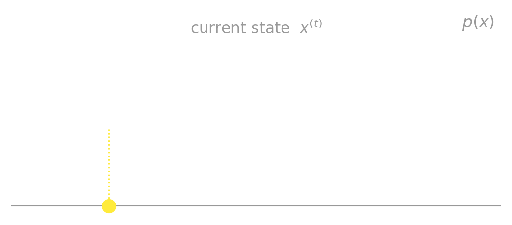
We want to sample this multimodal \(p(x)\). The chain sits at the current state.

この多峰性 \(p(x)\) から標本を取りたい。連鎖は現在の状態にいる。

Sibling-slide build-up (not fragments) so it reads as animation. Slide 1: just the current point on the target. ~20s.

MH, step by step (2/3)MH、一歩ずつ (2/3)

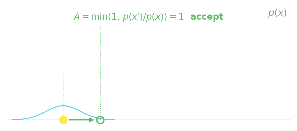
Propose a nearby move. It’s uphill (\(p(x') > p(x)\)), so the ratio \(p(x')/p(x) > 1\) and \(A=\min(1,\cdot)=1\) — always accept.

近くへの移動を提案。上り（\(p(x') > p(x)\)）なので比 \(p(x')/p(x) > 1\)、\(A=\min(1,\cdot)=1\) — 必ず受理。

Slide 2: a proposal that goes uphill. A=1, accept. The chain climbs toward high- density regions naturally. ~20s.

MH, step by step (3/3)MH、一歩ずつ (3/3)

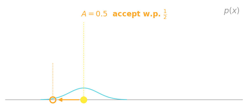
A downhill proposal (here \(p(x')/p(x)=0.5\)): \(A=0.5\) — accept only half the time. Sometimes the chain moves to lower density; that’s what lets it explore, not just hill-climb.

下りの提案（ここでは \(p(x')/p(x)=0.5\)）：\(A=0.5\) — 半分だけ受理。低密度へ動くこともある。それが、ただの山登りでなく探索を可能にする。

Slide 3: downhill, A=0.5, sometimes accept. The “sometimes accept downhill” is why MCMC samples the WHOLE distribution instead of converging to the mode. The 6th anim frame (reject, far/low-density) is in reserve if you want a 4th slide. ~20s.

Gibbs samplingギブズサンプリング

When you can sample each variable given the rest, resample one coordinate at a time:

\[x_i^{(t+1)} \sim P(x_i \mid x_{-i})\]

\(x_{-i}\) = all the other coordinates (everything except \(x_i\)).

• No accept/reject — every move is accepted.
• Moves are axis-aligned (one coordinate at a time).

Preview: in the Kemp sampler the \(\theta_i\) step is pure Gibbs (conjugate); the hyperparameters need Metropolis.

各変数を他を固定して引けるとき、1座標ずつ再サンプリング：

\[x_i^{(t+1)} \sim P(x_i \mid x_{-i})\]

\(x_{-i}\) = 他のすべての座標（\(x_i\) 以外）。

• 受理／棄却なし — すべての移動を受理。
• 移動は軸に沿う（1座標ずつ）。

予告：Kempサンプラーでは \(\theta_i\) ステップは純粋なギブズ（共役）；超パラメータにはメトロポリスが要る。

Define x_{-i}. Gibbs always accepts -> the contrast with MH. The L-shaped moves in the figure. Plant the Kemp preview here. ~2 min.

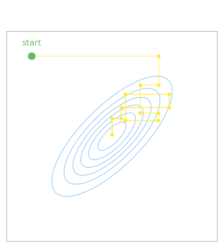
MH vs GibbsMH 対 ギブズ

Metropolis–Hastings

• works for any target
• propose + accept/reject
• needs only the ratio \(P(x')/P(x)\)
• proposal variance must be tuned

メトロポリス・ヘイスティングス

• どんな目標でも使える
• 提案 + 受理／棄却
• 比 \(P(x')/P(x)\) だけで足りる
• 提案の分散は調整が必要

Gibbs

• needs the conditionals \(P(x_i\mid x_{-i})\)
• always accepts
• one coordinate at a time
• no tuning, but can mix slowly

ギブズ

• 条件付き分布 \(P(x_i\mid x_{-i})\) が必要
• 常に受理
• 1座標ずつ
• 調整不要だが混合が遅いことも

Two-column structural parallel. The “proposal variance must be tuned” bullet sets up the interactive viz. ~1 min.

Poll — does the starting point matter?ポール — 出発点は関係ある?

You run your MH chain from two very different starting points, for a long time. The histograms of visited states are…

MHの連鎖をまったく違う2つの出発点から、長時間走らせる。訪れた状態のヒストグラムは…

• A. the same — the chain forgets where it started
• B. different — the start determines the answer
• C. depends on the proposal

• A. 同じ — 連鎖は出発点を忘れる
• B. 違う — 出発点が答えを決める
• C. 提案分布次第

A — an ergodic chain forgets its start and converges to \(\pi\) = the target. That’s the whole point of MCMC. …if it has mixed — which is exactly what the next demo is about. A — エルゴード的な連鎖は出発点を忘れ、\(\pi\)＝目標へ収束する。それがMCMCの核心。…ただし混合していれば — それこそ次のデモの主題。

Source: SP25 Markov-chains quiz Q4 (start-doesn’t-matter), recast as an MCMC convergence intuition. The “if it mixed” caveat is the deliberate hook into the viz. ~1 min.

Interactive: Gibbs & Metropolis–Hastingsインタラクティブ：ギブズとMH

Live demo — what to watchライブデモ — 注目点

A multimodal 2-D Gaussian mixture. We control the proposal variance and watch the acceptance ratio and mixing.

• σ too small → acceptance ≈ 1, but a slow random walk — stuck in one mode.
• σ too large → almost everything rejected, acceptance ≈ 0 — chain frozen.
• σ just right → acceptance ≈ 0.2–0.5, the chain explores.
• The catch → even good local acceptance can’t cross between well-separated modes.

多峰性の2次元ガウス混合。提案の分散を操作し、受理率と混合を観察する。

• σ が小さすぎ → 受理率 ≈ 1 だが遅いランダムウォーク — 1つの峰に閉じ込められる。
• σ が大きすぎ → ほぼ全て棄却、受理率 ≈ 0 — 連鎖が凍りつく。
• σ がちょうど良い → 受理率 ≈ 0.2〜0.5、連鎖が探索する。
• 落とし穴 → 局所の受理率が良くても、離れた峰の間は渡れない。

This slide just lists the beats; the demo does the work. Run the 5-demo script in widgets/README.md: Gibbs baseline -> tiny sigma -> huge sigma -> just-right -> trapped finale. The trapped demo is the punchline: acceptance ~0.6 but “modes visited 1/4”. ~30s on this slide, then switch to the demo.

Gibbs & MH demoギブズとMHのデモ

THE interactive slide. background-interactive=true is required or the sliders won’t respond. Drive the 5-demo script live. If the iframe fails to load, skip to the next slide (static fallback) and narrate over the mh-anim + gibbs-trace figures from Block 5.

If the live demo isn’t availableライブデモが使えないとき

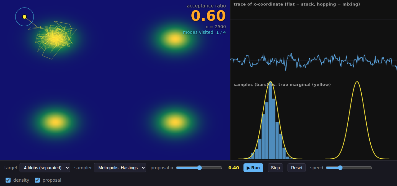
Trapped MH: acceptance is healthy (0.60) but only 1 of 4 modes was visited — the histogram fills just one peak. Good local acceptance ≠ good global mixing. Open week07.html to drive it live.

閉じ込められたMH：受理率は健全（0.60）だが4峰のうち1峰しか訪れていない — ヒストグラムは1峰だけ。良い局所受理率 ≠ 良い大域混合。week07.html を開けばライブで操作できる。

This is the static still for the PDF export (decktape can’t capture the live iframe). In the live HTML deck, step past it. It also doubles as the Poll 3 reference image. ~10s.

Poll — two runs disagreeポール — 2回の結果が食い違う

Two MH runs on the bimodal target give very different histograms after 1,000 steps. What went wrong?

二峰性の目標へのMH 2回が、1,000ステップ後にまったく違うヒストグラムになる。何が起きた?

• A. neither chain has mixed — each got stuck in a different mode
• B. MCMC is biased — this is expected
• C. the target has no stationary distribution

• A. どちらの連鎖も混合していない — それぞれ別の峰に閉じ込められた
• B. MCMCは偏っている — 想定内
• C. 目標に定常分布が存在しない

A — poor mixing, not bias. Both chains are ergodic in theory (each would reach \(\pi\) eventually), but with a local proposal neither has crossed between modes in 1,000 steps — so each chain reflects only the mode it started in, and the two disagree. That disagreement is the diagnostic: run several chains from different starts; if they don’t agree, none has mixed. A — 偏りではなく混合不良。両連鎖とも理論上はエルゴード的（各々いずれ \(\pi\) に達する）だが、局所提案では1,000ステップで峰の間を渡れず、各連鎖は出発した峰しか反映しないため、2つが食い違う。この食い違いこそ診断材料： 異なる出発点から複数の連鎖を走らせ、一致しなければどれも混合していない。

Source: SP25 Markov-chains stationary-distribution item, recast from “compute pi” to “did the sampler actually reach pi?”. Lands AFTER the demo showed a stuck chain. ~1 min.

Break休憩

Programmable inference (GenJAX)プログラム可能な推論（GenJAX）

One picture: classical method ⇄ GenJAX一枚で：古典的手法 ⇄ GenJAX

Classical

• basic Monte Carlo
• rejection sampling
• importance sampling
• K-particle IS / SMC
• particle filter
• MCMC / Metropolis–Hastings

古典的手法

• 基本のモンテカルロ
• 棄却サンプリング
• 重点サンプリング
• K粒子IS／SMC
• 粒子フィルタ
• MCMC／メトロポリス・ヘイスティングス

GenJAX surface

• simulate + vmap
• filter simulate by the constraint
• importance → (trace, log_weight)
• smc.ImportanceK(Target(…), k=N)
• smc.* chained over observations
• assemble it from update / assess

GenJAXの実体

• simulate + vmap
• 制約で simulate をフィルタ
• importance → (trace, log_weight)
• smc.ImportanceK(Target(…), k=N)
• 観測にわたる smc.* の連鎖
• update / assess から自分で組む

The idea: probabilistic programming gives you importance sampling for free, and hands you the scoring primitive (assess) to assemble MCMC — exactly what we’ll do for the Kemp model.

要点： 確率的プログラミングは重点サンプリングを無料で与え、MCMCを組み立てるための採点演算（assess）を渡す — まさにKempモデルでやること。

The LIGHT GenJAX summary — always runs. The thesis line is the hinge into Block 9. Note: MCMC is NOT a black box in genjax 0.10.3 (the repo’s pinned version) — you build it. Newer upstream (v1.0.10) adds hmc()/chain(); name-drop only. ~2 min. At rehearsal: show this OR the deep-dive (7b), maybe not both.

Deep-dive (1/4): the target and the skeleton詳説 (1/4)：目標と骨組み

@gen
def model():
    mu = normal(0.0, 1.0) @ "mu"   # prior
    y  = normal(mu, 0.5)  @ "y"    # likelihood
    return y

# score log p(mu, y=1.5) with assess
def log_p(mu):
    ch = C["mu"].set(mu).at["y"].set(1.5)
    logp, _ = model.assess(ch, ())
    return logp

• Goal: sample \(\mu\) from its posterior after seeing \(y = 1.5\).
• We pick one tool: assess — it returns \(\log p(\mu, y)\) for any \(\mu\).
• Every MH step is the same 3 lines: propose → score → accept. The only thing that changes is the proposal.

Closed-form posterior here is \(\mathcal{N}(1.2, 0.45)\) — so we can check the chain landed right.

• 目標： \(y = 1.5\) を見た後の事後分布から \(\mu\) を標本する。
• 道具は1つ：assess — 任意の \(\mu\) に \(\log p(\mu, y)\) を返す。
• どのMHステップも同じ3行：提案 → 採点 → 受理。変わるのは提案分布だけ。

ここでの閉形式事後分布は \(\mathcal{N}(1.2, 0.45)\) — だから連鎖が正しく収束したか確認できる。

7b deep-dive, slide 1 of 4. HEAVY/fenced — show OR skip for the summary. Target: mu~N(0,1), y~N(mu,0.5), observe y=1.5 -> posterior N(1.2, 0.447). The ONE primitive is assess (= log joint). The recurring skeleton is propose/score/accept; only the proposal changes. assess matches the closed form exactly (verified, mh_genjax.py). ~1.5 min.

Deep-dive (2/4): proposal A — a random walk詳説 (2/4)：提案A — ランダムウォーク

def mh_step_A(key, mu, sigma=0.5):
    kp, ka = random.split(key)
    mu_new = mu + sigma * random.normal(kp)  # propose
    logA = log_p(mu_new) - log_p(mu)         # score
    ok = jnp.log(random.uniform(ka)) < logA  # accept?
    return jnp.where(ok, mu_new, mu)

start mu=0.0,  log_p=-5.65
propose mu'=0.266   logA=+1.42 → accept ✓
# uphill (closer to 1.2) ⇒ logA>0 ⇒ always accept

• Random-walk proposal: \(\mu' = \mu + \sigma\,\varepsilon\), a small Gaussian step.
• It’s symmetric (\(q(\mu'\!\mid\mu)=q(\mu\!\mid\mu')\)), so the \(q\) terms cancel and \(\log A\) is just the score difference — the animation’s rule.
• Run 4000 steps: mean \(1.17\), accept rate 0.68. Small steps, mostly accepted.

This is the workhorse proposal — the one in the interactive demo.

• ランダムウォーク提案： \(\mu' = \mu + \sigma\,\varepsilon\)、小さなガウスのステップ。
• 対称（\(q(\mu'\!\mid\mu)=q(\mu\!\mid\mu')\)）なので \(q\) が打ち消え、\(\log A\) はただのスコア差 — アニメの規則。
• 4000ステップ実行：平均 \(1.17\)、受理率 0.68。小さなステップ、ほぼ受理。

これが主力の提案 — インタラクティブデモのもの。

7b slide 2 of 4. Proposal A = symmetric random walk. Because it’s symmetric the q-ratio is 1, so logA = log_p(new) - log_p(old) — literally the animation’s accept rule. Real numbers (mh_genjax.py, key=1): from mu=0, propose 0.266, logA=+1.42, accept. Chain: mean 1.17 (true 1.2), accept 0.68. ~1.5 min.

Deep-dive (3/4): proposal B — independent jumps詳説 (3/4)：提案B — 独立ジャンプ

def mh_step_B(key, mu):
    kp, ka = random.split(key)
    mu_new = random.normal(kp)        # propose ~ N(0,1)
    logA = ( log_p(mu_new) - log_p(mu)
        + log_q(mu) - log_q(mu_new) )  # +q-correction!
    ok = jnp.log(random.uniform(ka)) < logA
    return jnp.where(ok, mu_new, mu)

propose mu'=-2.378  logA=-25.6 → reject ✗
# jumped away from the posterior ⇒ logA≪0 ⇒ reject

• Independent proposal: draw \(\mu' \sim \mathcal{N}(0,1)\) fresh — ignore where you are.
• The proposal is symmetric as a bell curve, but the kernel isn’t: since it ignores \(\mu\), the forward and reverse probabilities differ, \(q(\mu'\!\mid\mu)=\mathcal{N}(\mu';0,1) \neq \mathcal{N}(\mu;0,1)=q(\mu\!\mid\mu')\). So you must add \(\log q(\mu) - \log q(\mu')\) — drop it and the chain targets the wrong distribution.
• Run 4000 steps: mean \(1.23\), accept rate 0.25. Bold jumps, often rejected.

• 独立提案： \(\mu' \sim \mathcal{N}(0,1)\) を新たに引く — 現在地を無視。
• 提案は釣鐘型としては対称だが、カーネルは非対称：\(\mu\) を無視するため順方向と逆方向の確率が異なり、\(q(\mu'\!\mid\mu)=\mathcal{N}(\mu';0,1) \neq \mathcal{N}(\mu;0,1)=q(\mu\!\mid\mu')\)。だから \(\log q(\mu) - \log q(\mu')\) を加える必要がある — 省くと連鎖は誤った分布を狙う。
• 4000ステップ実行：平均 \(1.23\)、受理率 0.25。大胆なジャンプ、しばしば棄却。

7b slide 3 of 4. Proposal B = independent draw from the prior. THE teaching contrast: the q-correction term log q(mu) - log q(mu_new) appears — the ONLY new code vs. proposal A. PRECISION POINT (a student asked): N(0,1) is a symmetric distribution, but the MH symmetry that matters is KERNEL symmetry, q(mu’|mu)=q(mu|mu’). The independent proposal ignores mu, so q(mu’|mu)=N(mu’;0,1) =/= N(mu;0,1)=q(mu|mu’) — forward and reverse probabilities differ, hence the correction doesn’t cancel. (The random walk q(mu’|mu)=N(mu;mu,sigma) depends on mu’-mu and IS kernel-symmetric because the Gaussian is even.) Drop the correction -> wrong stationary dist. Real numbers (key=3): propose -2.378, logA=-25.6, reject. Chain: mean 1.23, accept 0.25 (vs A’s 0.68). ~2 min.

Deep-dive (4/4): same skeleton, your choice of proposal詳説 (4/4)：同じ骨組み、提案はあなた次第

	A: random walk	B: independent
propose	\(\mu + \sigma\varepsilon\)	\(\mu' \sim \mathcal{N}(0,1)\)
\(q(\mu'\!\mid\mu)=q(\mu\!\mid\mu')\)?	yes	no
\(q\)-correction	none	required
accept rate	0.68	0.25
post. mean	1.17	1.23

• Both land on the truth (\(\mu\approx 1.2\)) — MH is correct for any valid proposal.
• The proposal only changes efficiency: how often you accept, how fast you mix.
• The accept/reject rule never changed — only the proposal slotted into the skeleton did.

This is programmable inference: no black-box mh() in 0.10.3 — you assemble it, and you choose the proposal. (For Kemp, the proposal is a Gaussian step on \((\varphi,\log\kappa)\) — slide 60+.)

• どちらも真値に収束（\(\mu\approx 1.2\)）— MHは妥当な提案ならどれでも正しい。
• 提案が変えるのは効率だけ：受理頻度、混合の速さ。
• 受理／棄却の規則は不変 — 骨組みに差し込む提案だけが変わった。

これがプログラム可能な推論：0.10.3にブラックボックスの mh() はない — 自分で組み、提案を選ぶ。（Kempでは提案は \((\varphi,\log\kappa)\) 上のガウスステップ — スライド60〜。）

7b slide 4 of 4 — the payoff. BOTH proposals give the correct posterior (mean ~1.2): MH is exact for ANY valid proposal; the proposal only sets efficiency (accept rate / mixing speed). The accept rule was identical in A and B — only the proposal function changed. Hinge into Kemp: there the proposal is a Gaussian RW on (phi, log kappa). This whole 7b block is the on-ramp to the assignment. Cut the whole block under time pressure (show the LIGHT summary instead). ~2 min.

MCMC with People人を使ったMCMC

What if a person is the accept step?人が受理ステップだったら?

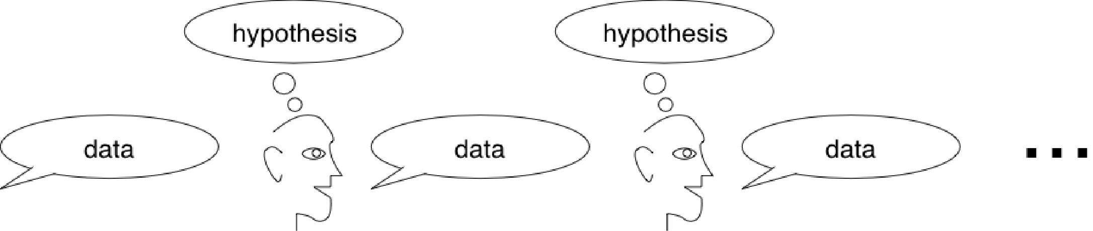
Show someone two stimuli — “which looks more like a cat?” — and treat their choice as the Metropolis accept/reject decision.

The chain alternates: a hypothesis in the head produces data (a response), which the next person reads as data and forms a new hypothesis.

2つの刺激を見せ — 「どちらがネコらしい?」 — その選択をメトロポリスの受理／棄却とみなす。

連鎖は交互に進む：頭の中の仮説がデータ（反応）を生み、次の人がそれをデータとして読み、新しい仮説を作る。

Show-before-tell. COSMOS s31. The human IS the accept step. This is the required reading (Sanborn & Griffiths). ~1.5 min.

The chain converges to the prior in their heads連鎖は頭の中の事前分布へ収束する

If learners sample from their posterior \(P(h\mid d) \propto P(d\mid h)\,P(h)\), then the Markov chain on hypotheses converges to the prior \(P(h)\) — the inductive biases in their heads.

You can read out someone’s prior by running them as an MCMC chain. (Bartlett 1932; Kirby 2001; Griffiths & Kalish 2007; Sanborn et al. 2010)

学習者が事後分布から標本を取る \(P(h\mid d) \propto P(d\mid h)\,P(h)\) なら、仮説上のマルコフ連鎖は事前分布 \(P(h)\) へ収束する — 頭の中の帰納バイアス。

人をMCMC連鎖として走らせれば、その事前分布を読み出せる。 (Bartlett 1932; Kirby 2001; Griffiths & Kalish 2007; Sanborn et al. 2010)

COSMOS s33/34. The deep payoff: iterated learning = a Markov chain on hypotheses whose stationary distribution is the prior. Connect to structure/process/behavior (Marr). ~2 min.

Recovering mental prototypes心的プロトタイプの復元

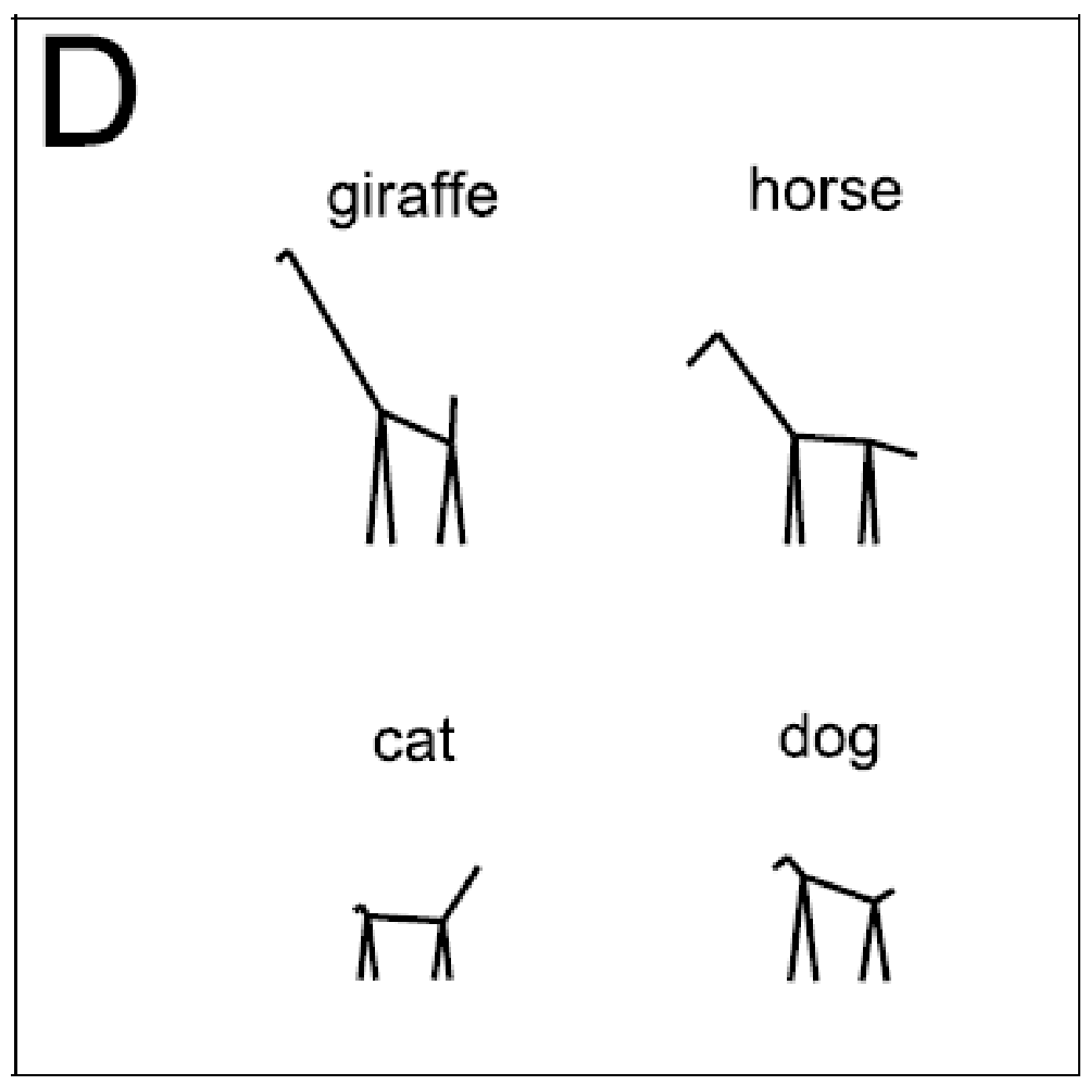
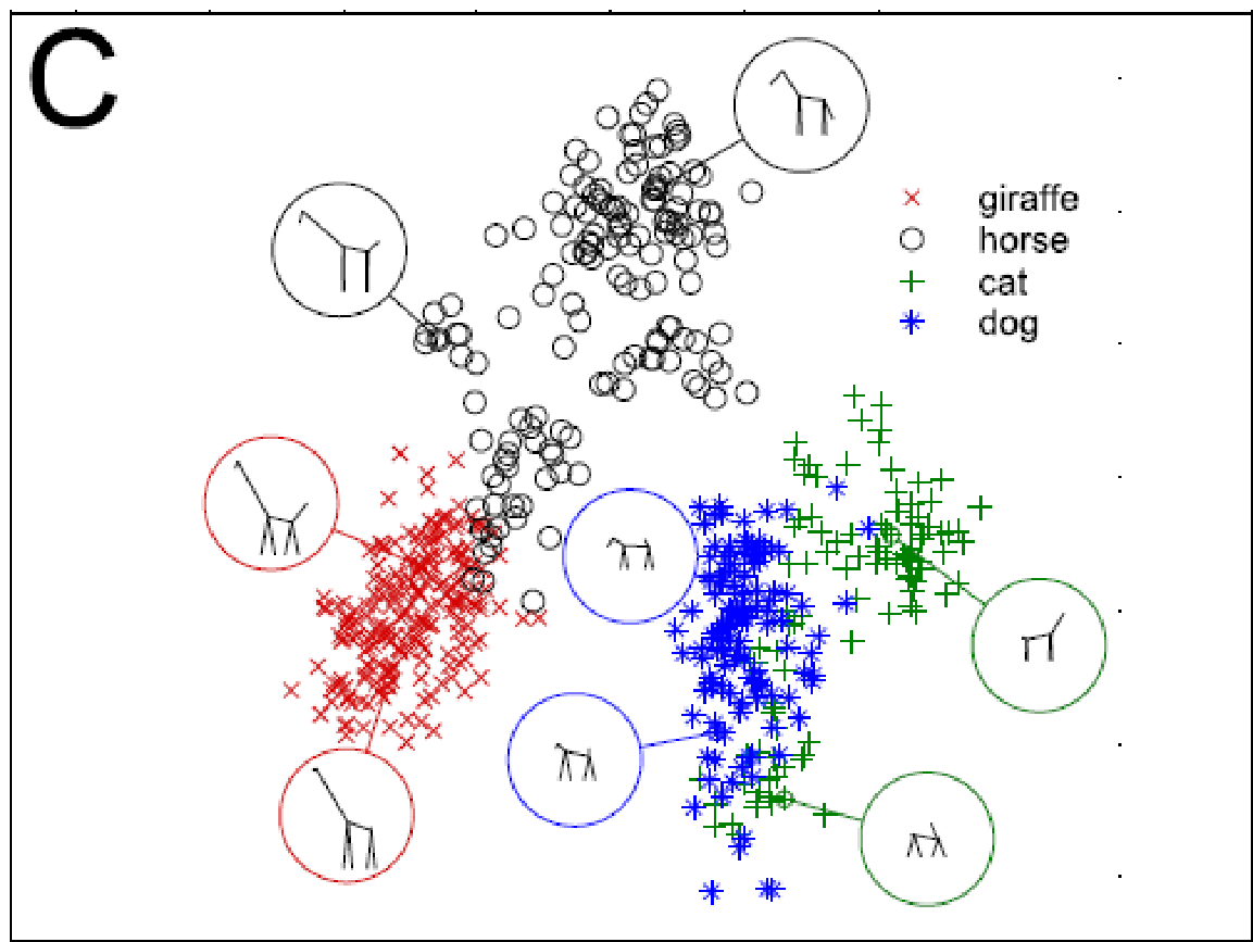
Sanborn & Griffiths (2007): MCMCP over a 9-D stick-figure space recovers each category’s mental prototype — giraffe, horse, cat, dog separate cleanly.

Sanborn & Griffiths (2007)：9次元の棒人形空間でのMCMCPが、各カテゴリの心的プロトタイプを復元 — キリン・ウマ・ネコ・イヌがきれいに分離。

COSMOS s36-38. The result figure. The 2-D scatter shows the four categories separating, with prototype morphs circled. ~1.5 min. Compression path: under time pressure, this slide + the cartoon + one sentence = the whole block in ~3 min. Optional extension (subjective-randomness ladders, music Gibbs) lives in images/cosmos_src/subj_random_ladder*.png — add only with a luxurious 12 min.

A sampler for the Kemp hierarchyKemp階層モデルのサンプラー

The model — from Week 4モデル — 第4週から

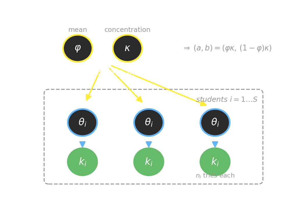
Each student \(i\) has a tonkatsu rate \(\theta_i \sim \text{Beta}(a,b)\); we observe counts \(k_i \sim \text{Binomial}(n_i, \theta_i)\).

The hyperparameters \((a,b)\) are unknown and learned — the overhypotheses. (Kemp, Perfors & Tenenbaum 2007 — no DPMM here.)

We’ll learn them through the mean \(\varphi=\tfrac{a}{a+b}\) and concentration \(\kappa=a+b\) (the figure’s top nodes) — easier to put priors on.

各学生 \(i\) はトンカツ率 \(\theta_i \sim \text{Beta}(a,b)\)；観測はカウント \(k_i \sim \text{Binomial}(n_i, \theta_i)\)。

超パラメータ \((a,b)\) は未知で学習する — オーバー仮説。(Kemp, Perfors & Tenenbaum 2007 — ここではDPMMなし。)

平均 \(\varphi=\tfrac{a}{a+b}\) と集中度 \(\kappa=a+b\)（図の上のノード）を通して学習する — 事前分布を置きやすい。

Callback to Week 4 Variant B. The hierarchy students already saw conceptually — now we give it a sampler. ~1.5 min.

Why we need a samplerなぜサンプラーが必要か

The joint posterior \(p(a, b, \{\theta_i\} \mid \text{data})\) has no clean closed form.

The textbook (T3 Ch 12) used importance sampling over the Beta-Binomial marginal — but with a broad hyperprior, most sampled \((a,b)\) explain the data poorly, so the estimate wobbles. The “blunt tool.”

Now we build the sharp one: a chain that spends its samples where the posterior mass actually is.

同時事後分布 \(p(a, b, \{\theta_i\} \mid \text{data})\) にはきれいな閉形式がない。

教科書（T3 第12章）はベータ二項周辺分布に重点サンプリングを使った — だが超事前分布が広いと、引いた \((a,b)\) の大半はデータをうまく説明せず、推定が揺れる。「鈍い道具」。

今、鋭い道具を作る：事後分布の質量が実際にある所に標本を使う連鎖。

Callback to the Block 3 “blunt tool” poll. This is the motivation for the whole block. ~1.5 min.

The recipe — two steps per sweepレシピ — 1スイープに2ステップ

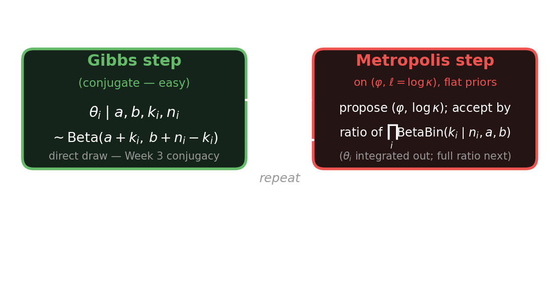
One half is free (conjugate Gibbs); the other half needs Metropolis. Alternate them. (\(\text{BetaBin}\) = the Beta-Binomial marginal likelihood — defined in two slides.)

片方は無料（共役ギブズ）；もう片方はメトロポリスが要る。交互に行う。（\(\text{BetaBin}\) = ベータ二項周辺尤度 — 2枚先で定義。）

The overview figure. Next two slides expand each half. ~1 min.

Step 1 — Gibbs the \(\theta_i\) (free)ステップ1 — \(\theta_i\) をギブズ（無料）

Hold \((a,b)\) fixed. Each student’s rate has a conjugate update — exactly Week 3:

\((a,b)\) を固定。各学生の率は共役更新 — まさに第3週：

\[\theta_i \mid a, b, k_i, n_i \;\sim\; \text{Beta}(a + k_i,\; b + n_i - k_i)\]

A direct draw — no rejection, no tuning. You’ve had this since Week 3 conjugacy: prior \(\text{Beta}(a,b)\) + \(k_i\) successes in \(n_i\) tries → posterior \(\text{Beta}(a+k_i, b+n_i-k_i)\).

直接引く — 棄却なし、調整なし。第3週の共役性で既習：事前 \(\text{Beta}(a,b)\) + \(n_i\) 回中 \(k_i\) 成功 → 事後 \(\text{Beta}(a+k_i, b+n_i-k_i)\)。

The easy half. Stress that they already know this from Week 3 — it’s just conjugacy in a loop. ~2 min.

Integrate out \(\theta_i\): the Beta-Binomial marginal\(\theta_i\) を積分消去：ベータ二項周辺分布

To score the hyperparameters \((a,b)\), we don’t want each \(\theta_i\) in the way — so average it out (the marginal likelihood of a student’s count):

\[\text{BetaBin}(k\mid n,a,b) = \int_0^1 \underbrace{\text{Binomial}(k\mid n,\theta)}_{\text{likelihood}}\;\underbrace{\text{Beta}(\theta\mid a,b)}_{\text{prior}}\,d\theta = \binom{n}{k}\,\frac{B(a+k,\; b+n-k)}{B(a,b)}\]

\(\binom{n}{k}\) = the binomial coefficient (“\(n\) choose \(k\)”). \(B(\alpha,\beta)\) = the Beta function, the normalizing constant of \(\text{Beta}(\alpha,\beta)\). Because Beta-Binomial is conjugate (Week 3), this integral is closed-form — no sampling needed. This is why \(\theta_i\) vanishes from the accept ratio.

超パラメータ \((a,b)\) を採点するとき、各 \(\theta_i\) が邪魔 — だから積分で消す（ある学生のカウントの周辺尤度）：

\[\text{BetaBin}(k\mid n,a,b) = \int_0^1 \underbrace{\text{Binomial}(k\mid n,\theta)}_{\text{尤度}}\;\underbrace{\text{Beta}(\theta\mid a,b)}_{\text{事前}}\,d\theta = \binom{n}{k}\,\frac{B(a+k,\; b+n-k)}{B(a,b)}\]

\(\binom{n}{k}\) = 二項係数（「\(n\) 個から \(k\) 個」）。\(B(\alpha,\beta)\) = ベータ関数、\(\text{Beta}(\alpha,\beta)\) の正規化定数。ベータ二項は共役（第3週）なので、この積分は閉形式 — サンプリング不要。だから受理比から \(\theta_i\) が消える。

NEW slide (added after round-1 student review flagged BetaBin as undefined). This is the missing piece for the assignment’s Metropolis step: shows what the marginal IS (the formula), names the Beta function B, and shows the integrate-out move that makes theta_i disappear. ~2 min.

Step 2 — Metropolis the hyperparameters: proposeステップ2 — 超パラメータをメトロポリス：提案

\((a,b)\) are not conjugate to anything. Reparametrize to mean and concentration, and work in \((\varphi,\, \ell)\) where \(\ell=\log\kappa\):

\[\varphi = \frac{a}{a+b} \in (0,1), \qquad \kappa = a + b > 0, \qquad \ell = \log\kappa\]

• Priors: flat (uniform) on both \(\varphi\in(0,1)\) and \(\ell\) (improper-flat — no bounds to track, so the prior ratio is exactly 1). Flat on \(\ell=\log\kappa\) is the log-uniform prior on \(\kappa\) — spans orders of magnitude.
• Propose a symmetric Gaussian step on each (tune the two widths separately):

\[\varphi' = \varphi + \epsilon_\varphi,\quad \epsilon_\varphi\sim\mathcal{N}(0,\sigma_\varphi^2); \qquad \ell' = \ell + \epsilon_\ell,\quad \epsilon_\ell\sim\mathcal{N}(0,\sigma_\ell^2)\]

• Map back to evaluate the model: \(\;\kappa' = e^{\ell'},\;\; a' = \varphi'\kappa',\;\; b' = (1-\varphi')\kappa'\).
• If \(\varphi'\notin(0,1)\) the flat prior is \(0\) ⇒ reject (set \(A=0\)). \(\sigma_\varphi,\sigma_\ell\) = the proposal widths you tune for mixing — the demo’s knob.

\((a,b)\) は何にも共役でない。平均と集中度に再パラメータ化し、\((\varphi,\,\ell)\) で扱う（\(\ell=\log\kappa\)）：

\[\varphi = \frac{a}{a+b} \in (0,1), \qquad \kappa = a + b > 0, \qquad \ell = \log\kappa\]

• 事前分布： \(\varphi\in(0,1)\) と \(\ell\) の両方に平坦（一様）（非正則平坦 — 境界を追う必要がなく、事前比はちょうど1）。\(\ell=\log\kappa\) に平坦 = \(\kappa\) に対数一様 — 桁にわたる。
• 各々に対称ガウスのステップで提案（2つの幅は別々に調整）：

\[\varphi' = \varphi + \epsilon_\varphi,\quad \epsilon_\varphi\sim\mathcal{N}(0,\sigma_\varphi^2); \qquad \ell' = \ell + \epsilon_\ell,\quad \epsilon_\ell\sim\mathcal{N}(0,\sigma_\ell^2)\]

• モデル評価のため逆写像：\(\;\kappa' = e^{\ell'},\;\; a' = \varphi'\kappa',\;\; b' = (1-\varphi')\kappa'\)。
• \(\varphi'\notin(0,1)\) なら平坦事前分布は \(0\) ⇒ 棄却（\(A=0\)）。\(\sigma_\varphi,\sigma_\ell\) = 混合のため調整する提案幅 — デモのつまみ。

Step 2a — the proposal. Split from the accept ratio (round-3 student review: the single slide was too dense and under-specified). Key adds: TWO sigmas (phi and ell need different step sizes), the inverse map to (a,b), and the out-of-support rule (phi’ outside (0,1) -> reject, because flat prior = 0). ~2 min.

Step 2 — Metropolis: the accept ratioステップ2 — メトロポリス：受理比

The general Metropolis–Hastings ratio has four factors. With this choice, three of them are \(1\):

\[A = \min\!\left(1,\; \underbrace{\frac{\prod_i \text{BetaBin}(k_i\mid n_i, a', b')}{\prod_i \text{BetaBin}(k_i\mid n_i, a, b)}}_{\text{marginal likelihood}}\;\times\;\underbrace{\frac{\pi(\varphi',\ell')}{\pi(\varphi,\ell)}}_{=\,1\ \text{(flat)}}\;\times\;\underbrace{\frac{q(\varphi,\ell\mid\varphi',\ell')}{q(\varphi',\ell'\mid\varphi,\ell)}}_{=\,1\ \text{(symmetric)}}\;\times\;\underbrace{J}_{=\,1\ \text{(no transform)}}\right)\]

\(a'=\varphi'\kappa',\; b'=(1-\varphi')\kappa',\; \kappa'=e^{\ell'}\) — the proposed hyperparameters (from the previous slide).

• prior ratio \(=1\): both priors are flat in \((\varphi,\ell)\).
• proposal ratio \(=1\): the Gaussian step is symmetric.
• Jacobian \(J=1\): the prior lives on the same coordinates \((\varphi,\ell)\) we sample in — no change of variables. If you instead put a flat prior on \((a,b)\) and sampled in \((\varphi,\ell)\), you would owe a Jacobian. Defining the prior in the sampling coordinates avoids it.

So \(A\) collapses to just the marginal-likelihood ratio. The \(\binom{n_i}{k_i}\) in each BetaBin is constant in \((a,b)\), so it cancels too — drop it. Note: this step scores \((a,b)\) through the marginal, so the \(\theta_i\) you just drew in the Gibbs step are not used here — they’re integrated out.

一般のメトロポリス・ヘイスティングス比は4因子。この選び方では3つが \(1\)：

\[A = \min\!\left(1,\; \underbrace{\frac{\prod_i \text{BetaBin}(k_i\mid n_i, a', b')}{\prod_i \text{BetaBin}(k_i\mid n_i, a, b)}}_{\text{周辺尤度}}\;\times\;\underbrace{\frac{\pi(\varphi',\ell')}{\pi(\varphi,\ell)}}_{=\,1\ \text{(平坦)}}\;\times\;\underbrace{\frac{q(\varphi,\ell\mid\varphi',\ell')}{q(\varphi',\ell'\mid\varphi,\ell)}}_{=\,1\ \text{(対称)}}\;\times\;\underbrace{J}_{=\,1\ \text{(変換なし)}}\right)\]

\(a'=\varphi'\kappa',\; b'=(1-\varphi')\kappa',\; \kappa'=e^{\ell'}\) — 提案された超パラメータ（前スライドより）。

• 事前比 \(=1\)： 両事前分布は \((\varphi,\ell)\) で平坦。
• 提案比 \(=1\)： ガウスのステップは対称。
• ヤコビアン \(J=1\)： 事前分布をサンプリングと同じ \((\varphi,\ell)\) 座標に置く — 変数変換なし。もし \((a,b)\) に平坦事前分布を置いて \((\varphi,\ell)\) でサンプリングすると、ヤコビアンが必要になる。サンプリング座標で事前分布を定義すれば回避できる。

よって \(A\) は周辺尤度の比だけになる。各 BetaBin の \(\binom{n_i}{k_i}\) は \((a,b)\) について定数なので打ち消え、省ける。注： このステップは周辺分布で \((a,b)\) を採点するので、ギブズで引いたばかりの \(\theta_i\) は使わない — 積分消去されている。

Step 2b — the accept ratio, now shown IN FULL (round-3 student review: the “no prior / no Jacobian” claim was load-bearing but buried in dim text, and a student couldn’t verify it or would code it wrong with a different parametrization). The four-factor form makes explicit WHY only the marginal survives under this exact (phi, log-kappa) + flat-prior + symmetric-Gaussian choice. Also notes the binomial coefficient cancels. ~2 min.

In GenJAX: the sampler you assembleGenJAXでは：自分で組むサンプラー

The recipe

• \(\theta_i\) step: direct \(\text{Beta}\) draw
• \((\varphi,\kappa)\) step: MH on the marginal
• alternate, collect samples after burn-in

burn-in = the early samples, discarded so the chain can forget its start (Week 6’s mixing) and reach \(\pi\) before you count.

レシピ

• \(\theta_i\) ステップ：直接 \(\text{Beta}\) から引く
• \((\varphi,\kappa)\) ステップ：周辺分布へMH
• 交互に行い、バーンイン後に標本収集

バーンイン = 初期の標本。連鎖が出発点を忘れ（第6週の混合）\(\pi\) に達するまで捨てる。

In GenJAX

• Gibbs step → beta(a+k, b+n-k).sample
• MH step → score the closed-form BetaBin (slide 52) directly — not the model’s joint assess, which would still contain \(\theta_i\).
• the MH skeleton is the deep-dive’s mh_step. The assignment builds this same chain a slightly different way — next slide.

GenJAXでは

• ギブズステップ → beta(a+k, b+n-k).sample
• MHステップ → 閉形式の BetaBin（スライド52）を直接採点 — モデルの同時 assess ではない（それは \(\theta_i\) を含む）。
• MHの骨格は詳説の mh_step。課題は同じ連鎖を少し違うやり方で作る — 次のスライド。

The chain spends its samples where the mass is — sharp. Importance sampling weighted a cloud of prior draws — blunt. Same model, better tool.

連鎖は質量のある所に標本を使う — 鋭い。重点サンプリングは事前draw群を重み付けた — 鈍い。同じモデル、より良い道具。

Two-column math | GenJAX. The closing contrast (sharp vs blunt) resolves the arc. Point them at the assignment stencil. ~2 min.

Two ways to score the same chain同じ連鎖を採点する2つの方法

This lecture — collapsed

\[A \propto \frac{\prod_i \text{BetaBin}(k_i\mid n_i, a', b')}{\prod_i \text{BetaBin}(k_i\mid n_i, a, b)}\]

• \(\theta_i\) integrated out (closed form)
• flat prior on \(\ell=\log\kappa\)
• the elegant shortcut — fewest moving parts

この講義 — 周辺化

\[A \propto \frac{\prod_i \text{BetaBin}(k_i\mid n_i, a', b')}{\prod_i \text{BetaBin}(k_i\mid n_i, a, b)}\]

• \(\theta_i\) を積分消去（閉形式）
• \(\ell=\log\kappa\) に平坦事前分布
• エレガントな近道 — 部品が最少

The assignment — explicit

\[\log A = \sum_i \log\tfrac{\text{Beta}(\theta_i\mid a',b')}{\text{Beta}(\theta_i\mid a,b)} + \log\tfrac{p(\ell')}{p(\ell)}\]

• scores the \(\theta_i\) you just drew in the Gibbs step
• weak proper \(\log\)-normal prior on \(\kappa\) (a real prior ratio)
• you see Gibbs and Metropolis working together

課題 — 明示的

\[\log A = \sum_i \log\tfrac{\text{Beta}(\theta_i\mid a',b')}{\text{Beta}(\theta_i\mid a,b)} + \log\tfrac{p(\ell')}{p(\ell)}\]

• ギブズで今引いた \(\theta_i\) を採点
• \(\kappa\) に弱い正則 \(\log\)-正規事前分布（本物の事前比）
• ギブズとメトロポリスが協働する様子が見える

Same chain, same target \(\pi\) — they just differ in what you condition on. Collapsing \(\theta_i\) gives lower-variance hyperparameter moves (less Monte-Carlo noise per step); keeping \(\theta_i\) is more general — it’s what you do the moment a step isn’t conjugate and you can’t integrate by hand. The assignment uses the explicit form so you build both moves yourself.

Does the choice matter for what’s learned? The answer (the posterior over the overhypothesis) is identical either way. But lower variance per step means the collapsed chain pins down \((\varphi,\kappa)\) in fewer sweeps — it learns the overhypothesis faster per unit of compute. That’s the only sense in which the sampler choice touches learning here: speed, not conclusion.

同じ連鎖、同じ目標 \(\pi\) — 違うのは何で条件付けるかだけ。\(\theta_i\) を周辺化すると超パラメータの動きが低分散（毎ステップのモンテカルロ雑音が減る）；\(\theta_i\) を保つ方が一般的 — ステップが共役でなく手で積分できない瞬間にこれを使う。課題は明示形を使い、両方の動きを自分で組む。

この選択は学習結果に影響するか? 結論（オーバー仮説の事後分布）はどちらでも同一。ただし毎ステップの分散が低いと、周辺化した連鎖はより少ないスイープで \((\varphi,\kappa)\) を絞り込む — 計算量あたり、オーバー仮説をより速く学習する。 サンプラーの選択が学習に触れるのはこの意味だけ：速さであって結論ではない。

NEW bridge slide (the deck’s accept ratio and the assignment’s accept ratio are NOT the same expression; a note-taker would code the wrong one). Left = what the previous slides built (marginal/collapsed, flat prior). Right = what the assignment PDF asks for (Gibbs-sampled theta scored with the Beta likelihood + a proper log-normal kappa prior). The yellow line is the actual teaching point and answers “why does the sampling choice matter”: collapsing = Rao-Blackwell, lower variance but needs a closed-form integral; keeping theta = general, the only option when conjugacy fails. Both target the same posterior. ~2 min. If tight, state the one sentence and move on – the assignment footnote carries it.

Wrapping upまとめ

The toolkit ladder道具立ての梯子

• Monte Carlo — average samples to estimate an expectation.
• Importance sampling — sample the wrong distribution, reweight.
• Particle filter — importance sampling, updated over time.
• MCMC (MH + Gibbs) — design a chain whose stationary distribution is your target.
• Applied: read out a person’s prior (MCMCP); learn the Kemp hierarchy’s hyperparameters.

Each rung bought a sharper tool for a harder target.

Why this still matters in 2026. You’ll rarely hand-write an accept ratio again — but the sample → score → reweight-or-accept loop didn’t go away, it got a learned proposal. A diffusion model is a learned reverse-MCMC; RLHF samples from a policy and reweights by a reward; best-of-\(N\) is importance sampling. The mechanics you built today are the conceptual core of how today’s models are trained, steered, and aligned.

• モンテカルロ — 標本を平均して期待値を推定。
• 重点サンプリング — 間違った分布から引き、重みで直す。
• 粒子フィルタ — 時間更新する重点サンプリング。
• MCMC（MH + ギブズ） — 定常分布が目標になる連鎖を設計。
• 応用： 人の事前分布を読み出す（MCMCP）；Kemp階層の超パラメータを学習。

各段が、より難しい目標へのより鋭い道具をもたらした。

なぜ2026年でも重要か。 受理比を手で書くことはもう滅多にない — だがサンプル→採点→重み付け／受理のループは消えず、学習された提案分布を得た。拡散モデルは学習された逆MCMC；RLHFは方策から引いて報酬で重み付け；best-of-\(N\) は重点サンプリング。今日組んだ仕組みは、現代のモデルが訓練・操舵・整合される仕方の概念的中核。

Recap. Then: the GenJAX sampling exercise (Kemp sampler) is the capstone. ~1 min.

Next week + the assignment来週 + 課題

• Assignment: build the Kemp sampler — Gibbs the \(\theta_i\), Metropolis the \((\varphi,\kappa)\). Stencil + Colab on the assignments page.
• Week 8: signal detection theory, MDPs, reinforcement learning — from inferring beliefs to choosing actions.

• 課題： Kempサンプラーを作る — \(\theta_i\) をギブズ、\((\varphi,\kappa)\) をメトロポリス。ひな形とColabは課題ページに。
• 第8週： 信号検出理論、MDP、強化学習 — 信念の推論から行動の選択へ。

Close. Confirm the Week 8 presenter against readings_map.yml. ~1 min.