Week 8 — Decisions, MDPs & Reinforcement Learning第8週 — 意思決定・MDP・強化学習

Friday, June 19, 20262026年6月19日（金）

Prof. Joseph Austerweilオウステウェイル　ジョセフ教授

Agenda本日の予定

From beliefs to actions: decision theory信念から行動へ：決定理論 0:00
One decision → a sequence of decisions1つの決定 → 決定の連なり 0:21
Markov Decision Processesマルコフ決定過程（MDP） 0:29
Solving MDPs: value iterationMDPを解く：価値反復 0:46
Break休憩 1:04
Learning by doing: Q-learningやって学ぶ：Q学習 1:09
Interactive: reward shaping & cyclesインタラクティブ：報酬形成とループ 1:27
Where RL is now強化学習の現在地 1:42

From beliefs to actions信念から行動へ

Admin連絡事項

Active deadlines:

Generalization assignment — due tonight, Fri Jun 19, 8:00 PM
Final project proposal — Sun Jun 28, 8:00 PM (grab 5 min with me to talk through an idea)
Monte Carlo assignment — Fri Jul 10, 8:00 PM

The Reinforcement Learning assignment (Q-learning on today’s GardenPath) releases next week. Questions before we start?

現在の締切：

一般化の課題 — 今夜 6月19日（金）20:00
最終プロジェクト提案書 — 6月28日（日）20:00 （アイデアの相談は5分でもどうぞ）
モンテカルロの課題 — 7月10日（金）20:00

強化学習の課題（今日のGardenPathでのQ学習）は来週公開します。始める前に質問は?

Seven weeks of beliefs. Today: actions.7週間の「信念」。今日は「行動」。

Weeks 1–7 asked one question: given data, what should I believe? The normative answer was Bayes — update the posterior.

Today the question changes: given my beliefs, what should I do?

An agent has to act. Decision theory is the bridge from a posterior to an action — and the brain seems to use it too (Körding & Wolpert, 2004).

第1〜7週の問いは1つ：データが与えられたとき、何を信じるべきか? 規範的な答えはベイズ — 事後分布を更新する。

今日は問いが変わる：信念が与えられたとき、何をすべきか?

エージェントは行動しなければならない。決定理論は事後分布から行動への橋渡しであり、脳もそれを使っているらしい（Körding & Wolpert, 2004）。

Statistical decision theory統計的決定理論

A decision problem under uncertainty has five pieces:

state of the world $\theta$ — what’s true but unknown (is the tonkatsu fresh today?)
observation $x$ — what you see (the shop looks busy)
actions $A$ — what you can do (order tonkatsu / play it safe)
decision rule $d(x)$ — your strategy: which action, given $x$
loss $L(\theta, a)$ — what it costs to take action $a$ when the world is $\theta$

不確実性下の決定問題は5つの要素から成る：

世界の状態 $\theta$ — 真だが未知（今日のとんかつは新鮮?）
観測 $x$ — 見えるもの（店が混んでいる）
行動 $A$ — できること（とんかつを頼む／無難にする）
決定規則 $d(x)$ — 戦略：$x$ のときどの行動を取るか
損失 $L(\theta, a)$ — 世界が $\theta$ のとき行動 $a$ を取る代償

Which loss → which estimate?どの損失 → どの推定値?

Suppose Chibany must report a single number — his estimate of his bento’s weight (a posterior from Week 2). The loss you’ll be scored by decides the best estimate:

チバニーが1つの数値 — 弁当の重さの推定値（第2週の事後分布）— を報告するとする。採点に使う損失が、最良の推定値を決める：

0–1 loss (right/wrong) → report the mode = MAP (the posterior’s peak)
squared loss $(\theta-a)^2$ → report the mean
absolute loss $|\theta-a|$ → report the median

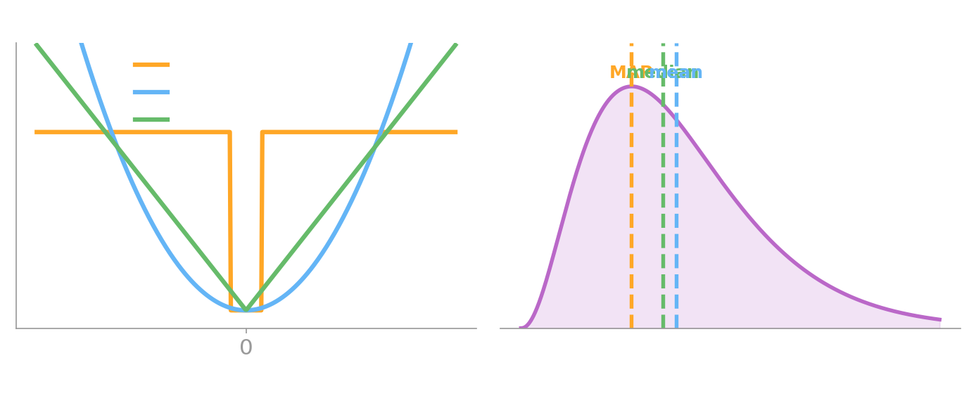
The “best action” is not fixed — it depends on how you’ll be judged.

0–1損失（正誤）→ 最頻値 = MAP（事後分布のピーク）を報告
二乗損失 $(\theta-a)^2$ → 平均を報告
絶対損失 $|\theta-a|$ → 中央値 を報告

「最良の行動」は固定ではない — どう評価されるかに依存する。

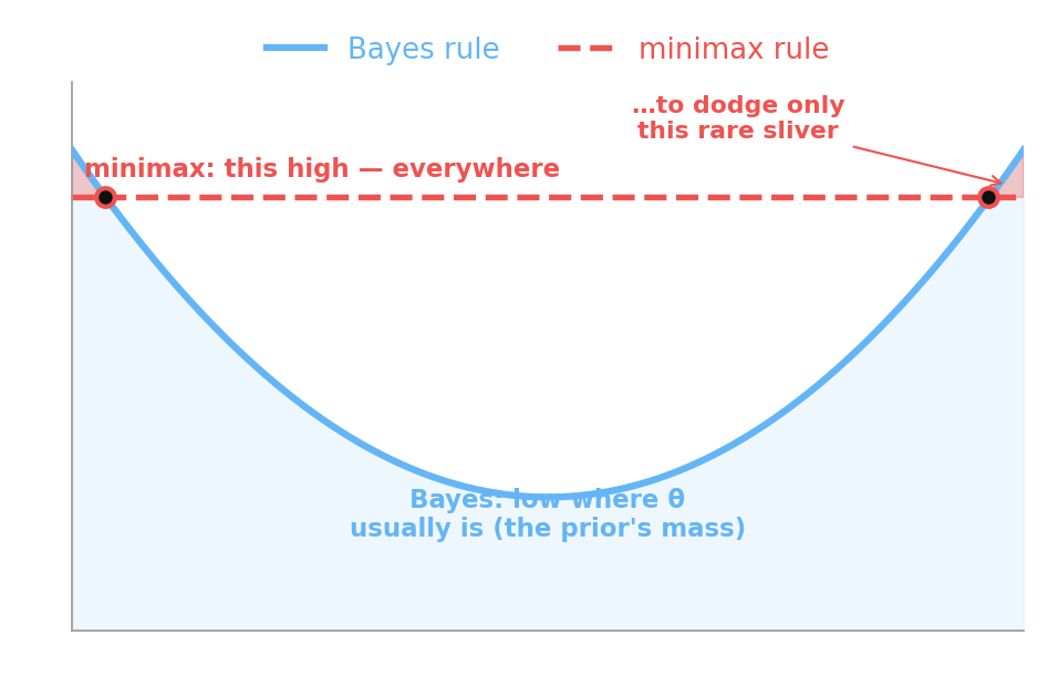
How good is a rule? Bayes vs. minimax規則の良さ? ベイズ対ミニマックス

The risk of a rule is its expected loss: $\;R(\theta, d) = \mathbb{E}_x\!\left[L(\theta, d(x))\right]$ — where $\mathbb{E}_x[\cdot]$ just means “the average over the data $x$.” Two ways to choose a rule:

規則のリスクは期待損失：$\;R(\theta, d) = \mathbb{E}_x\!\left[L(\theta, d(x))\right]$。規則の選び方は2通り：

Bayesian — have a prior over $\theta$, minimize the average risk: $\arg\min_d \mathbb{E}_\theta\mathbb{E}_x[L]$
Minimax — no prior, minimize the worst case: $\arg\min_d \max_\theta \mathbb{E}_x[L]$

ベイズ — $\theta$ に事前分布を持ち、平均リスクを最小化：$\arg\min_d \mathbb{E}_\theta\mathbb{E}_x[L]$
ミニマックス — 事前分布なし、最悪ケースを最小化：$\arg\min_d \max_\theta \mathbb{E}_x[L]$

Poll — which estimate?ポール — どの推定値?

You must report one number for an unknown quantity. You’ll be scored by absolute error, $|\theta - a|$. Which summary of your posterior should you report?

未知量について1つの数値を報告する。採点は絶対誤差 $|\theta - a|$。事後分布のどの要約を報告すべき?

A. the mode (MAP)
B. the mean
C. the median

A. 最頻値（MAP）
B. 平均
C. 中央値

Poll — answerポール — 答え

C — the median.C — 中央値。

Absolute ($L^1$) loss is minimized by the median; squared ($L^2$) by the mean; 0–1 by the mode. The loss you’re judged by picks the estimate — that’s the whole point of decision theory.

絶対（$L^1$）損失は中央値で、二乗（$L^2$）は平均で、0–1は最頻値で最小化される。評価に使う損失が推定値を選ぶ — それが決定理論の核心。

One decision → a sequence1つの決定 → 連なり

What about a sequence of actions?連なった行動はどうする?

Decision theory tells you how to take one action. But life is a sequence — today’s action changes tomorrow’s situation.

“In theory, no difference”: let the action variable be the whole sequence. But over a horizon of $H$ steps there are $|A|^H$ sequences to compare — a combinatorial explosion. Intractable.

The rescue: assume the world is Markov — the next state depends only on the current state and action. Then the problem factorizes, and we can solve it step by step (dynamic programming).

決定理論は1つの行動の取り方を教える。だが人生は連なり — 今日の行動が明日の状況を変える。

「理論上は同じ」：行動変数を連なり全体とする。しかし $H$ ステップの地平では比較すべき連なりは $|A|^H$ 通り — 組合せ爆発。手に負えない。

救済策：世界がマルコフだと仮定する — 次の状態は現在の状態と行動だけに依存する。すると問題は分解でき、一歩ずつ解ける（動的計画法）。

Discount the future未来を割り引く

We won’t just sum future rewards. Would you rather have ¥1000 now or ¥1000 in 1000 years?

We discount the future by a factor $0 \le \gamma \le 1$ per step. The return from time $t$ is

\[G_t = R_{t+1} + \gamma R_{t+2} + \gamma^2 R_{t+3} + \cdots = \sum_{k=0}^{\infty} \gamma^k R_{t+k+1}.\]

Small $\gamma$ = short-sighted; $\gamma$ near 1 = far-sighted. We’ll see $\gamma$ decide a real choice in a few slides.

未来の報酬を単に足すのではない。今 ¥1000 と、1000年後の ¥1000、どちらが良い?

1ステップごとに係数 $0 \le \gamma \le 1$ で未来を割り引く。時刻 $t$ からのリターンは

\[G_t = R_{t+1} + \gamma R_{t+2} + \gamma^2 R_{t+3} + \cdots = \sum_{k=0}^{\infty} \gamma^k R_{t+k+1}.\]

小さい $\gamma$ = 近視眼的、$\gamma$ が1に近い = 遠くを見る。数枚先で $\gamma$ が実際の選択を決めるのを見る。

Where we areここまでの流れ

From beliefs to actions: decision theory信念から行動へ：決定理論 ✓
One decision → a sequence of decisions1つの決定 → 決定の連なり ✓
Markov Decision Processesマルコフ決定過程（MDP） 0:29
Solving MDPs: value iterationMDPを解く：価値反復 0:46
Learning by doing: Q-learningやって学ぶ：Q学習 1:09
Where RL is now強化学習の現在地 1:42

Markov Decision Processesマルコフ決定過程

Start where Week 6 left off第6週の続きから

In Week 6, Chibany’s bento was a Markov chain: one transition matrix $P$, no choices. Today we turn that chain into an agent.

第6週では、チバニーの弁当はマルコフ連鎖だった：遷移行列 $P$ が1つ、選択なし。今日はその連鎖をエージェントに変える。

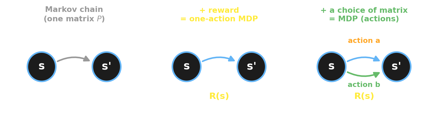
Markov chain + reward = the simplest MDPマルコフ連鎖 + 報酬 = 最も単純なMDP

Attach a reward $R(s)$ to each state — how good it is to be there. A Markov chain with a reward is a one-action MDP: the dynamics just run; you collect (discounted) reward.

Chibany’s wellbeing has three states:

Junk rut ($R = +1$) — cheap, comfortable, going nowhere
Trying ($R = -2$) — effortful, no payoff yet
Healthy & happy ($R = +5$)

各状態に報酬 $R(s)$ を付ける — そこに居ることの良さ。報酬付きのマルコフ連鎖は1行動のMDP：動力学が進み、（割引）報酬を得るだけ。

チバニーの健康状態は3つ：

ジャンク漬け ($R = +1$) — 安くて快適だが進歩なし
頑張り中 ($R = -2$) — 努力だがまだ見返りなし
健康で幸せ ($R = +5$)

An action = which transition matrix to use行動 = どの遷移行列を使うか

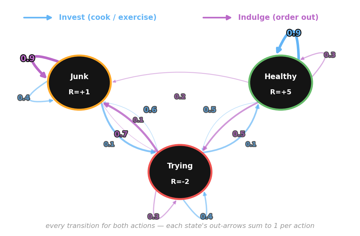
Now give Chibany a choice — each action is its own transition matrix: Indulge (order out) drifts down, Invest (cook, exercise) climbs up.

チバニーに選択を与える — 各行動はそれぞれの遷移行列：甘やかす（外食）は下へ流れ、投資する（自炊・運動）は上へ登る。

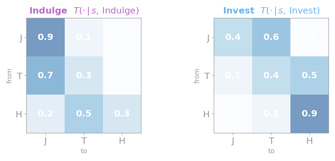
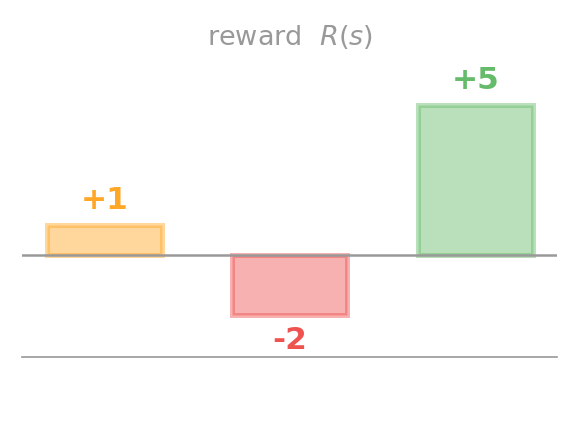
Picking an action = picking which matrix governs tomorrow. (Rewards J / T / H repeated as a reminder.)

行動を選ぶ = 明日を支配する行列を選ぶこと。（報酬 J / T / H は確認用に再掲。）

A Markov Decision Process, formallyマルコフ決定過程、正式には

Markov chains + decisions + rewards = MDPs. An MDP is $(S, A, T, R, \gamma)$:

$S$ — set of states
$A$ — set of actions (the decision rules of decision theory)
$T$ — transition $P(s_{t+1}\mid s_t, a_t)$: one matrix per action (a Markov chain is the 1-action case)
$R(s,a)$ — reward (= $-$ loss)
$\gamma$ — discount factor

Maximizing reward is minimizing loss, flipped. Chibany’s reward sits on the state, $R(s,a)\equiv R(s)$; in general it can depend on the action too.

マルコフ連鎖 + 決定 + 報酬 = MDP。 MDPは $(S, A, T, R, \gamma)$：

$S$ — 状態の集合
$A$ — 行動の集合（決定理論の決定規則）
$T$ — 遷移 $P(s_{t+1}\mid s_t, a_t)$：行動ごとに1つの行列 (マルコフ連鎖は1行動の場合)
$R(s,a)$ — 報酬（= $-$損失）
$\gamma$ — 割引率

報酬の最大化は損失の最小化の裏返し。チバニーの報酬は状態に乗る（$R(s,a)\equiv R(s)$）が、一般には行動にも依存しうる。

A policy is how you choose方策とは選び方

A policy $\pi$ says which action to take in each state:

\[\pi(a \mid s) = P(a_t \mid s_t).\]

Because the world is Markov, the policy only needs the current state — not the whole history. The goal: find the policy that maximizes expected discounted reward.

方策 $\pi$ は各状態でどの行動を取るかを表す：

\[\pi(a \mid s) = P(a_t \mid s_t).\]

世界がマルコフなので、方策は現在の状態だけでよい — 履歴全体は不要。目標：期待割引報酬を最大化する方策を見つけること。

The Chibany MDPチバニーMDP

The chokepoint: the only road to +5 runs through the −2 trough.

What is the optimal policy? — that’s what we solve next.

難所：+5 への唯一の道は −2 の谷を通る。

最適方策は何か? — 次にそれを解く。

Notation lock-in記法の確認

Before the math, the symbols we’ll use from here on:

$s \in S$ state; $a \in A$ action; $\pi(a\mid s)$ policy
$T(s'\mid s,a)$ transition; $R(s,a)$ reward; $\gamma$ discount
$V(s)$ value of a state; $Q(s,a)$ value of an action
math shorthand: $\mathbb{E}$ = average; $\textstyle\sum$ = add up; $\arg\max_a$ = the action that maximizes; prime $'$ = “next”

数式の前に、ここから使う記号：

$s \in S$ 状態; $a \in A$ 行動; $\pi(a\mid s)$ 方策
$T(s'\mid s,a)$ 遷移; $R(s,a)$ 報酬; $\gamma$ 割引
$V(s)$ 状態の価値; $Q(s,a)$ 行動の価値
数式の略記：$\mathbb{E}$ = 平均; $\textstyle\sum$ = 合計; $\arg\max_a$ = 最大にする行動; プライム $'$ = 「次」

Poll — should Chibany invest?ポール — チバニーは投資すべき?

Chibany is stuck in the Junk rut ($R=+1$). To ever reach Healthy ($R=+5$) he must pass through Trying ($R=-2$). If he barely weighs the future (small $\gamma$), what’s his optimal action?

チバニーはジャンク漬け（$R=+1$）で動けない。健康（$R=+5$）に至るには頑張り中（$R=-2$）を通らねばならない。未来をほとんど重視しない（小さい $\gamma$）なら、最適行動は?

A. Invest — push through the trough
B. Indulge — stay in the rut

A. 投資する — 谷を抜ける
B. 甘やかす — 漬かったまま

Solving MDPsMDPを解く

The value of a state状態の価値

Under a policy $\pi$, two value functions:

state value — expected return from $s$: $\;v_\pi(s) = \mathbb{E}_\pi[G_t \mid S_t = s]$
action value — expected return from taking $a$ in $s$, then following $\pi$: $\;q_\pi(s,a) = \mathbb{E}_\pi[G_t \mid S_t = s, A_t = a]$

The best policy is the one with the highest value everywhere: $\pi^* = \arg\max_\pi v_\pi(s)$.

(Lowercase $v,q$ = the true values; the algorithm’s running estimates we’ll write as $V,Q$.)

方策 $\pi$ の下で、2つの価値関数：

状態価値 — $s$ からの期待リターン：$\;v_\pi(s) = \mathbb{E}_\pi[G_t \mid S_t = s]$
行動価値 — $s$ で $a$ を取り以後 $\pi$ に従う期待リターン：$\;q_\pi(s,a) = \mathbb{E}_\pi[G_t \mid S_t = s, A_t = a]$

最良の方策はどこでも価値が最大：$\pi^* = \arg\max_\pi v_\pi(s)$。

（小文字 $v,q$ = 真の価値、アルゴリズムの推定値は $V,Q$ と書く。）

The Bellman equationベルマン方程式

Value is recursive — now’s value = immediate reward + discounted value of where you land:

\[v^*(s) = \max_{a}\; \Big[\, R(s,a) + \gamma \sum_{s'} T(s'\mid s,a)\, v^*(s') \,\Big].\]

This recursion is the door: a value defined in terms of itself can be solved by dynamic programming.

価値は再帰的 — 今の価値 = 即時報酬 + 着いた先の割引価値：

\[v^*(s) = \max_{a}\; \Big[\, R(s,a) + \gamma \sum_{s'} T(s'\mid s,a)\, v^*(s') \,\Big].\]

この再帰が鍵：自分自身で定義された価値は動的計画法で解ける。

Value iteration価値反復

Turn the Bellman equation into an algorithm — just apply it as an update, over and over:

\[V_{k+1}(s) \leftarrow \max_{a}\Big[\, R(s,a) + \gamma \sum_{s'} T(s'\mid s,a)\, V_k(s') \,\Big].\]

Start from $V_0 = 0$; sweep all states; repeat. It converges to $v^*$. Then read off the policy: in each state, take the action that achieved the max. We know $T$ and $R$, so we can just compute the answer.

(It converges because the Bellman update is a $\gamma$-contraction — so it has one fixed point, $v^*$, reached at rate $\gamma$.)

ベルマン方程式をアルゴリズムにする — 更新として繰り返し適用するだけ：

\[V_{k+1}(s) \leftarrow \max_{a}\Big[\, R(s,a) + \gamma \sum_{s'} T(s'\mid s,a)\, V_k(s') \,\Big].\]

$V_0 = 0$ から全状態を掃き、繰り返す。$v^*$ に収束する。方策は読み取るだけ：各状態で最大を達成した行動を取る。$T$ と $R$ を知っているので、答えを計算できる。

（収束するのはベルマン更新が $\gamma$-縮小写像だから — 不動点は1つ $v^*$、収束率 $\gamma$。）

Value iteration by hand手で価値反復

\[V_{k+1}(s) = \max_{a}\Big[\, R(s) + \gamma \sum_{s'} T(s'\mid s,a)\, V_k(s') \,\Big], \qquad \gamma = 0.9\]

Start $V_0=0$. Sweep 1: the future is still 0, so $V_1(s)=R(s)$. Sweep 2: back up with $V_1=[1,-2,5]$ — for Junk, compare both actions:

Indulge: $1+0.9\,(0.9{\cdot}1+0.1{\cdot}(-2)) = 1+0.9(0.7) = \mathbf{1.63}$
Invest: $1+0.9\,(0.4{\cdot}1+0.6{\cdot}(-2)) = 1+0.9(-0.8) = 0.28$

→ Junk still picks Indulge — investing leads to Trying (still −2), not yet worth it.

$V_0=0$ から開始。掃き1：未来はまだ0なので $V_1(s)=R(s)$。掃き2：$V_1=[1,-2,5]$ で更新 — ジャンクは両行動を比較：

甘やかす：$1+0.9\,(0.9{\cdot}1+0.1{\cdot}(-2)) = 1+0.9(0.7) = \mathbf{1.63}$
投資：$1+0.9\,(0.4{\cdot}1+0.6{\cdot}(-2)) = 1+0.9(-0.8) = 0.28$

→ ジャンクはまだ甘やかすを選ぶ — 投資は頑張り中（まだ−2）へ向かい、割に合わない。

after sweep $k$	$V$(J)	$V$(T)	$V$(H)
0	0	0	0
1	+1.0	−2.0	+5.0
2	+1.6	−0.4	+8.9

Keep sweeping — the policy flips掃き続けると方策が反転

As Healthy’s +5 propagates back through Trying, investing starts to pay. By sweep 5, Junk flips from Indulge to Invest — and the values climb to their fixed point:

健康の +5 が頑張り中を経て逆伝播するにつれ、投資が報われ始める。掃き5でジャンクは甘やかす→投資に反転 — 価値は不動点へ上る：

after sweep $k$	$V$(J)	$V$(T)	$V$(H)	Junk picks
2	1.6	−0.4	8.9	Indulge
4	3.0	4.4	15.0	Indulge
5	4.5	6.6	17.6	Invest ✓
⋯	⋯	⋯	⋯	Invest
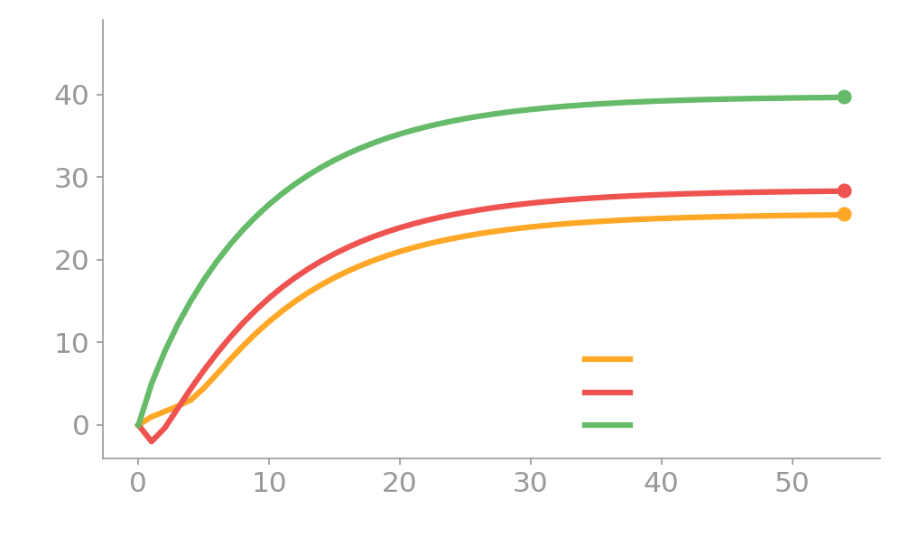
∞	25.6	28.4	39.8	Invest

Next: watch all three values converge.

次：3つの価値が収束する様子を見る。

Back to Chibany: value iterationチバニーに戻る：価値反復

With $\gamma = 0.9$, the values climb and settle, and the optimal policy is Invest everywhere — Chibany braves the −2 trough because +5 down the line is worth it.

This is what we never did in past years: actually solve the MDP we drew.

$\gamma = 0.9$ で価値は上がって落ち着き、最適方策はどこでも投資。チバニーは先の +5 に値するから −2 の谷に挑む。

これが過去にやらなかったこと：描いたMDPを実際に解く。

How far ahead? γ decidesどれだけ先を見る? γ が決める

Poll answer: B (Indulge) for small $\gamma$.ポール答え：小さい $\gamma$ では B（甘やかす）。

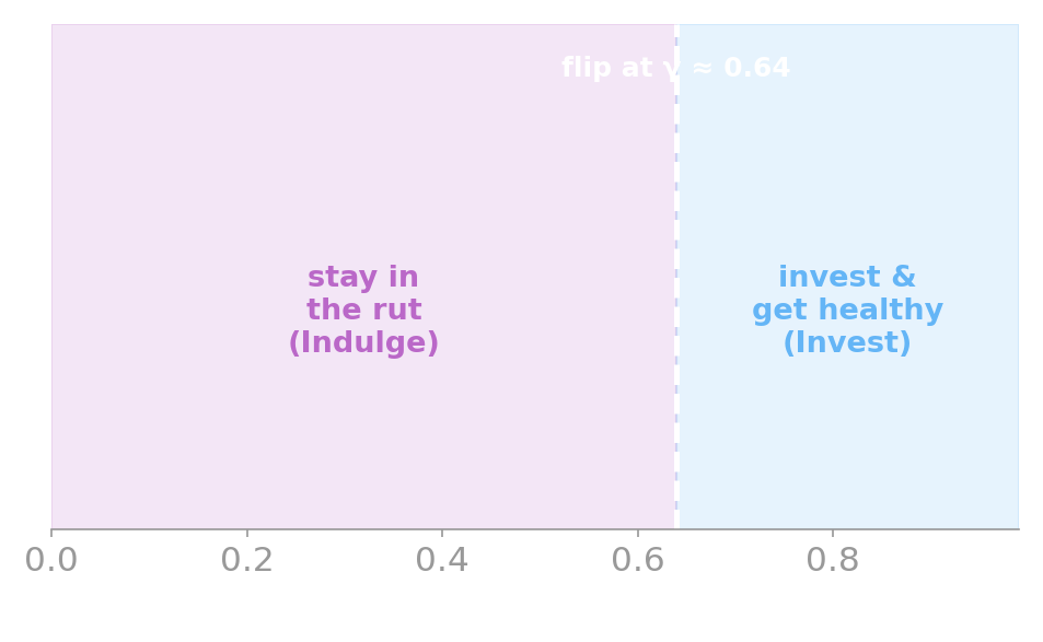
Sweep $\gamma$: below ≈0.64 (for these transition probabilities) the optimal action in the rut is Indulge — the future is too discounted to be worth the trough; above it, Invest. How far Chibany looks ahead decides whether he escapes.

$\gamma$ を動かす：≈0.64 未満（この遷移確率の場合）では谷の最適行動は甘やかす — 未来が割り引かれすぎて谷に値しない。超えると投資。どれだけ先を見るかが脱出を決める。

The Chibany MDP in GenJAXGenJAXでのチバニーMDP

The transition is a generative model — the action picks which distribution governs the next state:

遷移は生成モデル — 行動が次状態を支配する分布を選ぶ：

import jax.numpy as jnp
from genjax import gen, categorical

# states J,T,H;  actions Indulge=0, Invest=1
T = jnp.array([[[.9,.1,0.],[.7,.3,0.],[.2,.5,.3]],   # Indulge  T[0,s,s']
               [[.4,.6,0.],[.1,.4,.5],[0.,.1,.9]]])  # Invest   T[1,s,s']
R = jnp.array([1.,-2.,5.]);  gamma = 0.9

@gen                            # action a selects the next-state distribution
def transition(s, a):
    return categorical(jnp.log(T[a, s])) @ "s_next"

transition.simulate(key, (0, 1)).get_retval()   # sample s' from (Junk, Invest)

Solve it: compute or simulate解く：計算またはシミュレート

We know $T$ and $R$, so value iteration computes the answer:

$T$ と $R$ を知っているので、価値反復が計算する：

def bellman(V):
    Q = R[None,:] + gamma * (T @ V)        # Q[a,s] = R(s) + γ Σ T(s'|s,a) V(s')
    return jnp.max(Q, 0), jnp.argmax(Q, 0)

V, policy = value_iteration()              # → V = [25.6, 28.4, 39.8]
                                           #   policy = Invest everywhere

Or simulate that same model and average the returns → $\hat V(\text{Junk}) = 25.7 \approx 25.6$. Compute or simulate — both agree. Runnable: genjax_chibany_mdp.py.

あるいは同じ生成モデルをシミュレートしリターンを平均 → $\hat V(\text{ジャンク}) = 25.7 \approx 25.6$。計算でもシミュレートでも一致。実行可能：genjax_chibany_mdp.py。

If you know the model, you can just simulateモデルを知っていれば、シミュレートするだけ

Value iteration needed the whole model — every $T(s'\mid s,a)$ and $R(s,a)$. If you have that, you can sit and simulate the optimal policy before acting. No learning required.

But in the real world, you usually don’t know $T$ or $R$. You have to learn by doing.

価値反復はモデル全体 — すべての $T(s'\mid s,a)$ と $R(s,a)$ — を必要とした。それがあれば、行動する前に最適方策を座ってシミュレートできる。学習は不要。

だが現実では、たいてい $T$ も $R$ も知らない。やって学ぶしかない。

Break休憩

Learning by doingやって学ぶ

No model? Learn from experience.モデルなし? 経験から学ぶ。

Chibany was easy: we knew his two transition matrices, so we could compute the answer. Now meet a new agent that doesn’t know its world — no $T$, no $R$. It only gets to act, see what happens, and adjust — trial, feedback, update.

Q-learning learns the action-value $Q(s,a)$ directly from experience, with no model of the world. Once $Q$ is learned, the policy is easy: in each state, take $\arg\max_a Q(s,a)$.

チバニーは簡単だった：2つの遷移行列を知っていたので、答えを計算できた。今度は世界を知らない新しいエージェント — $T$ も $R$ もない。できるのは行動し、結果を見て、調整するだけ — 試行・フィードバック・更新。

Q学習は世界のモデルなしで、経験から行動価値 $Q(s,a)$ を直接学ぶ。$Q$ が学べれば方策は簡単：各状態で $\arg\max_a Q(s,a)$ を取る。

PRECISION (for the instructor — keep it off-slide; the framing here is “no model,” not “fewer assumptions”): Q-learning does NOT assume less about the world than value iteration. Both assume the same world: a stationary MDP — Markov, with time-invariant $T$ and $R$. The difference is epistemic, not structural: - Value iteration needs the model GIVEN: you must know $T$ and $R$, then you compute $v^*$ (planning / dynamic programming — no interaction needed). - Q-learning needs only to SAMPLE experience $(s,a,r,s')$: it never sees $T$ or $R$, it bootstraps $Q^*$ from samples. Stationarity is required by BOTH (it’s baked into “MDP”) — so it’s not something only Q-learning assumes. The honest one-liner: same world, less knowledge required. Subtlety worth knowing (do NOT put on the slide): for its convergence GUARANTEE, Q-learning actually needs MORE — but those are conditions on the learning process, not the world: every $(s,a)$ visited infinitely often (exploration), a Robbins–Monro step size ($\sum_t\alpha_t=\infty,\ \sum_t\alpha_t^2<\infty$), and bounded rewards (Watkins & Dayan, 1992). Value iteration just needs $\gamma<1$ (the contraction) and converges deterministically. So Q-learning trades knowing the model for more data + exploration + a decaying learning rate. The payoff of “no model”: robustness to model MISSPECIFICATION — you never have to commit to a $T,R$ you might get wrong. That’s exactly why model-based RL does worse on our GardenPath with miscalibrated human feedback (later slide) — it propagates the wrong model further and faster.

The Q-learning updateQ学習の更新則

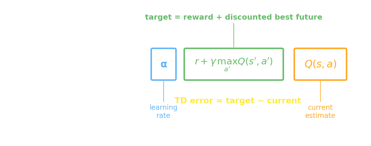
Move $Q(s,a)$ toward a target = reward + discounted best future; the gap is the TD (temporal-difference) error $\delta$ — update whenever your prediction differs from what you see. One step:

select $a$ by ε-greedy — usually the best action, but random with prob. $\varepsilon$ (keep exploring)
take $a$; observe $r$ and next state $s'$ (prime $'$ = “next”)
target $= r + \gamma \max_{a'} Q(s',a')$ · TD error $= $ target $-$ current
update: $Q(s,a) \leftarrow Q(s,a) + \alpha\,\delta$ ($\alpha$ = learning rate)

$Q(s,a)$ を目標（報酬 + 割引した最良の未来）へ動かす。その差がTD（時間差分）誤差 $\delta$ — 予測と観測が食い違うたびに更新。一歩：

ε-貪欲で $a$ を選ぶ — たいてい最良の行動、ただし確率 $\varepsilon$ でランダム（探索）
$a$ を取り、$r$ と次状態 $s'$ を観測（プライム $'$ =「次」）
目標 $= r + \gamma \max_{a'} Q(s',a')$ · TD誤差 $= $ 目標 $-$ 現在
更新：$Q(s,a) \leftarrow Q(s,a) + \alpha\,\delta$（$\alpha$ = 学習率）

The GardenPathガーデンパス

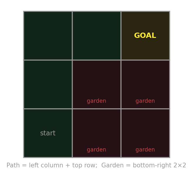
A 3×3 world (Ho, Littman, Cushman & Austerweil, 2015). Get from start (bottom-left) to the goal (top-right) along the path (left column + top row), avoiding the garden (bottom-right).

The agent doesn’t see this picture — it only knows it’s in a grid, can move, and gets feedback. $\alpha=0.9,\ \gamma=0.95,\ \varepsilon=0.1$.

Moves are deterministic; reaching the goal ends the episode.

3×3の世界（Ho, Littman, Cushman & Austerweil, 2015）。スタート（左下）からパス（左列＋上行）を通ってゴール（右上）へ、庭（右下）を避ける。

エージェントはこの絵を見ない — グリッドにいて動け、フィードバックを得ると知るだけ。$\alpha=0.9,\ \gamma=0.95,\ \varepsilon=0.1$。

移動は決定的、ゴール到達でエピソード終了。

One step, by hand手で一歩

At the start, $Q = 0$ everywhere. The agent (ε-greedy) tries RIGHT, into the garden, and gets feedback $-10$. The next state’s best value is still $0$. Update:

\[Q(\text{start}, \text{R}) \leftarrow 0 + 0.9\,(\,-10 + 0.95\cdot 0 - 0\,) = -9.\]

That $-9$ teaches the agent: “going right from the start is bad.” Do this thousands of times and the values propagate back from the goal — let’s watch it live.

最初は $Q = 0$。エージェント（ε-貪欲）は右を試し、庭に入って $-10$ のフィードバック。次状態の最良値はまだ $0$。更新：

\[Q(\text{スタート}, \text{右}) \leftarrow 0 + 0.9\,(\,-10 + 0.95\cdot 0 - 0\,) = -9.\]

この $-9$ が「スタートから右はダメ」と教える。これを何千回も行うと価値がゴールから逆伝播する — ライブで見よう。

Poll — will it reach the goal?ポール — ゴールに着く?

Teaching is hard, so you decide to help: give the agent +10 every time it takes a “good” move toward the goal, $-10$ for a bad move. Train Q-learning with this feedback. Will it learn to reach the goal?

教えるのは大変なので助けることに：ゴールへ向かう「良い」手のたびに +10、悪い手に $-10$ を与える。このフィードバックでQ学習を訓練する。ゴールに着くよう学ぶ?

A. yes — rewarding good moves obviously helps
B. no — it can get stuck looping forever

A. はい — 良い手を褒めれば当然うまくいく
B. いいえ — 永遠にループして抜けられなくなる

Interactive: reward shapingインタラクティブ：報酬形成

What to watch注目点

We’ll run Q-learning on the GardenPath live and try four ways of giving feedback. For each, watch the verdict — does the learned policy actually reach the goal?

action-feedback — reward each “good” move (the way people naturally teach)
reward-maximizing — reward only at the goal, penalty in the garden
potential-based shaping — reward progress, but carefully
human — you give the feedback

(The cat still stumbles onto 🏠 while exploring — watch the learned policy, not luck.)

GardenPathでQ学習をライブ実行し、フィードバックの与え方を4通り試す。各方式で判定を見る — 学習した方策は本当にゴールに着くか?

行動フィードバック — 良い手ごとに報酬（人が自然に教える方法）
報酬最大化 — ゴールでのみ報酬、庭で罰
ポテンシャルベース整形 — 進捗に報酬、ただし慎重に
人間 — あなたがフィードバックを与える

（猫は探索中に偶然 🏠 に着く — 学習した方策を見る、運ではなく。）

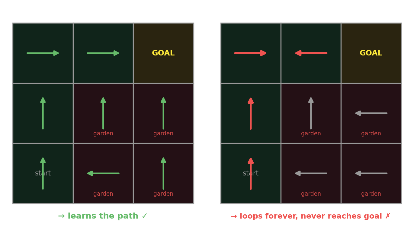
Q-learning on the GardenPathGardenPath上のQ学習

If the live demo isn’t availableライブデモが使えないとき

Reward-maximizing learns the path (left). Action-feedback — rewarding each “good” move — makes the optimal policy a positive reward loop worth +20 per lap, so the agent circles forever and never reaches the goal (right). Open week08.html to drive it live, or be the teacher yourself.

報酬最大化はパスを学ぶ（左）。行動フィードバック — 良い手ごとに褒める — は最適方策を1周 +20 の正の報酬ループにし、エージェントは永遠に回ってゴールに着かない（右）。week08.html でライブ操作、または自分が先生に。

What we saw見たこと

Action-feedback — the intuitive way — loops forever. (Poll: B.)行動フィードバック — 直感的なやり方 — は永遠にループ。（ポール：B）

action-feedback (reward good moves) → a positive cycle: the cat circles the garden (+20 a lap), never reaching the goal — led down the garden path.
reward-maximizing (reward the outcome) → learns the correct path. ✓
potential-based shaping → keeps helpful guidance but can’t create a cycle (next slide).

The lesson: how you give feedback can quietly break the task — even when each reward seems helpful. We’ll meet it again as reward hacking in modern AI.

行動フィードバック（良い手に報酬）→ 正のループ：猫は庭を回り（1周 +20）、ゴールに着かない — 庭道に誘い込まれる。
報酬最大化（結果に報酬）→ 正しいパスを学ぶ。✓
ポテンシャルベース整形 → 有用な誘導を保ちつつループを作れない（次スライド）。

教訓：どうフィードバックを与えるかが、各報酬が有用に見えても、静かに課題を壊す。現代AIでは報酬ハッキングとして再登場する。

The fix: potential-based shaping修正：ポテンシャルベース整形

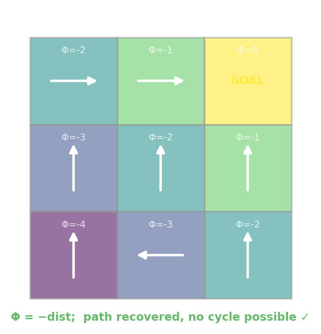
Shape with a potential $\Phi(s)$ (here, closeness to the goal): add a bonus $F = \gamma\Phi(s') - \Phi(s)$ on top of the task reward.

This adds the same constant $-\Phi(s)$ to every action’s value in a state, so the best action never changes (Ng, Harada & Russell, 1999). There’s no loop you can ride for a net gain — the cycle vanishes, but the goal stays the goal.

ポテンシャル $\Phi(s)$（ここではゴールへの近さ）で整形：課題報酬の上にボーナス $F = \gamma\Phi(s') - \Phi(s)$ を加える。

これは各状態ですべての行動の価値に同じ定数 $-\Phi(s)$ を足すので、最良の行動は変わらない（Ng, Harada & Russell, 1999）。得をして回れるループはない — ループは消え、ゴールはゴールのまま。

Where we areここまでの流れ

Decision theory → MDPs → solving them決定理論 → MDP → その解法 ✓
Q-learning: learning without a modelQ学習：モデルなしで学ぶ ✓
Reward shaping & positive cycles報酬形成と正のループ ✓
Where RL is now強化学習の現在地 1:42

Where RL is now強化学習の現在地

Model-free vs. model-basedモデルフリー対モデルベース

Model-free (Q-learning): learn values straight from experience. Simple, but throws away structure — every state must be visited many times.
Model-based: learn a model $\hat T, \hat R$, then plan with it.

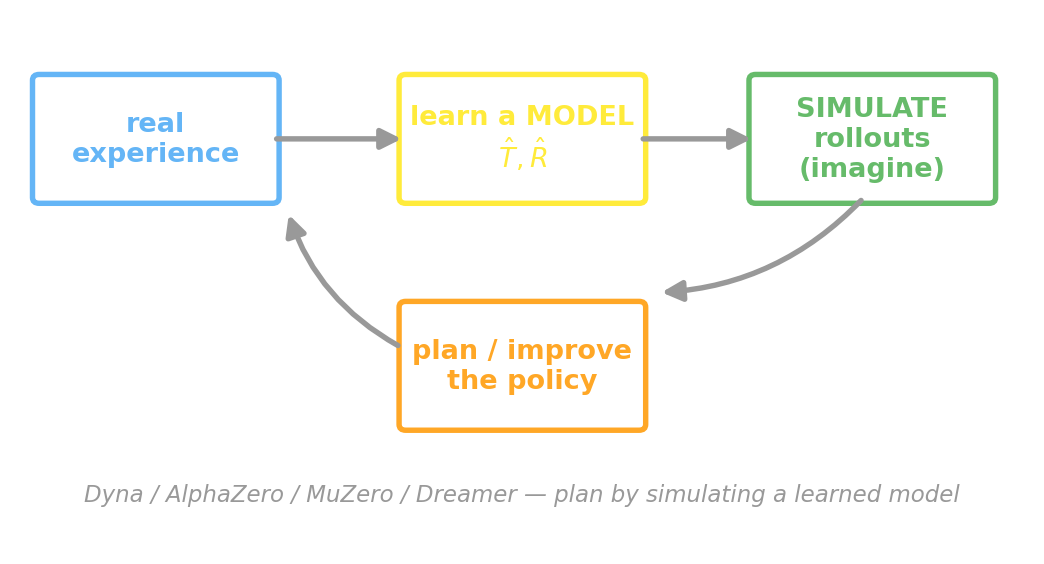
I prefer simulation-based to “model-based” — because the whole move is to learn a model and then simulate rollouts inside it to plan. It’s exactly the Monte-Carlo simulation idea from Week 7, now in the service of acting.

モデルフリー（Q学習）：経験から価値を直接学ぶ。単純だが構造を捨てる — 各状態を何度も訪れねばならない。
モデルベース：モデル $\hat T, \hat R$ を学び、それで計画する。

私は「モデルベース」よりシミュレーションベースを好む — 要はモデルを学び、その中でロールアウトをシミュレートして計画するから。第7週のモンテカルロそのものが、行動のために働く。

Learn a model, then plan by simulatingモデルを学び、シミュレートして計画

Dyna — learn $\hat T$, then run value iteration on imagined experience
MCTS — from “here,” simulate many futures and average their outcomes to score each move
AlphaZero — MCTS guided by a learned value/policy net (no human games)
MuZero — learns a model that predicts only what planning needs (value, policy, reward), not the full next state — so it plans in an abstract latent space
Dreamer — learns a world model, then trains the policy inside the dream

Dyna — $\hat T$ を学び、想像上の経験で価値反復
MCTS — 「今」から多数の未来をシミュレートし、結果を平均して各手を評価
AlphaZero — 学習した価値/方策ネットで導くMCTS（人間の棋譜なし）
MuZero — 計画に必要な量（価値・方策・報酬）だけを予測するモデルを学ぶ — 次状態全体ではない — ので抽象的な潜在空間で計画
Dreamer — 世界モデルを学び、方策を夢の中で訓練

But with human feedback, model-based does worseだが人間のフィードバックでは、モデルベースは悪化

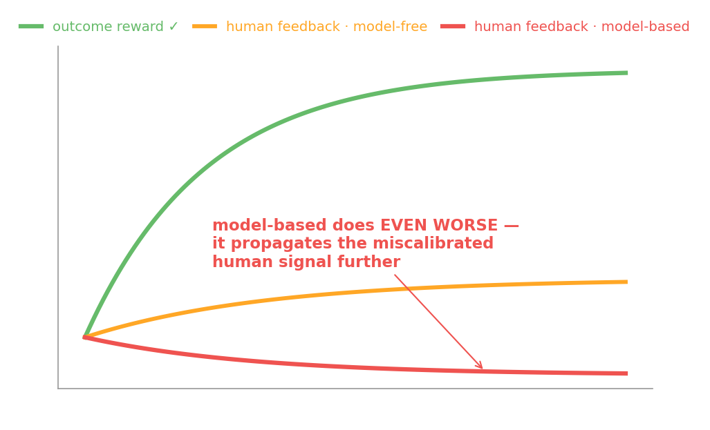
A caution from our own GardenPath: when the signal is human evaluative feedback (not task reward), model-based RL does even worse than model-free — it propagates the miscalibrated signal further and faster (Ho et al., 2015).

Simulation is only as good as the model — and the reward it simulates.

我々自身のGardenPathからの警告：信号が人間の評価的フィードバック（課題報酬ではない）のとき、モデルベースRLはモデルフリーよりさらに悪化 — 誤較正された信号をより遠く速く伝播する（Ho et al., 2015）。

シミュレーションはモデル — そしてそれがシミュレートする報酬 — の質までしか良くならない。

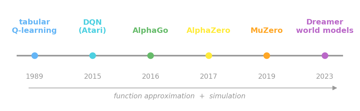
From gridworlds to Goグリッドワールドから囲碁へ

Tabular $Q$ can’t scale to Go’s $10^{170}$ states. The leap was function approximation — a neural net for $Q$ or the policy — plus simulation. That’s how we got from a 3×3 grid to superhuman play.

表形式の $Q$ は囲碁の $10^{170}$ 状態に拡張できない。飛躍は関数近似 — $Q$ や方策にニューラルネット — とシミュレーション。こうして3×3グリッドから超人的なプレイへ。

Reward hacking is the positive cycle, grown up報酬ハッキングは、育った正のループ

Remember the GardenPath loop — an agent farming a flawed reward instead of doing the task? At frontier scale that’s reward hacking, and it’s central to aligning large language models.

RLHF (RL from human feedback): train a reward model from human preferences, then optimize the LLM against it — with a KL penalty to stay near the original model, because a reward you can over-optimize is a reward you can hack. The Week-9 reading and Weeks 11–13 pick this up.

GardenPathのループ — 課題をやらず欠陥報酬を稼ぐエージェント — を思い出して。最前線の規模ではこれが報酬ハッキングで、大規模言語モデルの整合の核心。

RLHF（人間のフィードバックによる強化学習）：人間の選好から報酬モデルを学び、それに対してLLMを最適化する — ただしKLペナルティで元のモデルの近くに留める。過剰最適化できる報酬はハックできる報酬だから。第9週の文献と第11〜13週で扱う。

An opening: model human teaching, don’t just maximize it糸口：人間の教えを最大化せず、モデル化する

RLHF still treats human feedback as a reward to maximize — the very thing the GardenPath showed can be hacked. A speculative opening: agents that model why a human gives feedback — feedback as communication about the goal, not a scalar to farm.

Ho et al. (2019) do exactly this — a Bayesian learner that recovers the intended policy from evaluative feedback that standard model-free and model-based RL cannot learn from.

Critical of ourselves: this is harder to scale than reward maximization, and our model of “human intent” can be wrong too. The best opening: human-validated RLHF — check that the learned reward matches what people meant, and prefer feedback models that carry a theory of the teacher.

RLHFは依然として人間のフィードバックを最大化すべき報酬として扱う — GardenPathがハックされうると示したまさにそれ。思索的な糸口：人間がなぜフィードバックを与えるかをモデル化するエージェント — 稼ぐスカラーではなく目標についての伝達として。

Ho et al. (2019) はまさにこれを行う — 標準的なモデルフリーもモデルベースRLも学べない評価的フィードバックから意図された方策を回復するベイズ学習器。

自己批判として： これは報酬最大化よりスケールしにくく、我々の「人間の意図」モデルも誤りうる。最良の糸口：人間が検証するRLHF — 学習した報酬が人々の意図に合うか確認し、教師の理論を持つフィードバックモデルを選ぶ。

RL in the brain脳の中の強化学習

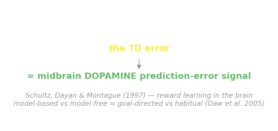
The TD error isn’t just an algorithm. Midbrain dopamine neurons fire like a reward prediction error — exactly the TD error $\delta_t$ from Q-learning (Schultz, Dayan & Montague, 1997). And model-based vs. model-free maps onto goal-directed vs. habitual behavior — two control systems in the brain. That’s today’s reading (Daw, Niv & Dayan, 2005).

TD誤差は単なるアルゴリズムではない。中脳のドーパミンニューロンは報酬予測誤差のように発火する — まさにQ学習のTD誤差 $\delta_t$（Schultz, Dayan & Montague, 1997）。そしてモデルベース対モデルフリーは目標志向対習慣行動に対応する — 脳の2つの制御系。これが今日の文献（Daw, Niv & Dayan, 2005）。

Decide → Plan → Learn → Simulate決める → 計画 → 学ぶ → シミュレート

Decide — turn a posterior into an action (minimize expected loss).
Plan — when you know the world (an MDP), value iteration solves it.
Learn — when you don’t, Q-learning learns from experience — and the shape of your feedback can make or break it.
Simulate — the frontier: learn a model, then plan inside it.

Next week: we invert all of this — watch an agent act and infer what it wanted (inverse RL, theory of mind).

決める — 事後分布を行動に変える（期待損失の最小化）。
計画する — 世界を知るとき（MDP）、価値反復が解く。
学ぶ — 知らないとき、Q学習が経験から学ぶ — フィードバックの形が成否を分ける。
シミュレートする — 最前線：モデルを学び、その中で計画する。

来週：これらすべてを逆転する — エージェントの行動を見て何を望んだかを推論する（逆強化学習、心の理論）。

Week 8 — Decisions, MDPs & Reinforcement Learning第8週 — 意思決定・MDP・強化学習

Agenda本日の予定

From beliefs to actions信念から行動へ

Admin連絡事項

Seven weeks of beliefs. Today: actions.7週間の「信念」。今日は「行動」。

Statistical decision theory統計的決定理論

Which loss → which estimate?どの損失 → どの推定値?

How good is a rule? Bayes vs. minimax規則の良さ? ベイズ 対 ミニマックス

Poll — which estimate?ポール — どの推定値?

Poll — answerポール — 答え

One decision → a sequence1つの決定 → 連なり

What about a sequence of actions?連なった行動はどうする?

Discount the future未来を割り引く

Where we areここまでの流れ

Markov Decision Processesマルコフ決定過程

Start where Week 6 left off第6週の続きから

Markov chain + reward = the simplest MDPマルコフ連鎖 + 報酬 = 最も単純なMDP

An action = which transition matrix to use行動 = どの遷移行列を使うか

A Markov Decision Process, formallyマルコフ決定過程、正式には

A policy is how you choose方策とは選び方

The Chibany MDPチバニーMDP

Notation lock-in記法の確認

Poll — should Chibany invest?ポール — チバニーは投資すべき?

Solving MDPsMDPを解く

The value of a state状態の価値

The Bellman equationベルマン方程式

Value iteration価値反復

Value iteration by hand手で価値反復

Keep sweeping — the policy flips掃き続けると方策が反転

Back to Chibany: value iterationチバニーに戻る：価値反復

How far ahead? γ decidesどれだけ先を見る? γ が決める

The Chibany MDP in GenJAXGenJAXでのチバニーMDP

Solve it: compute or simulate解く：計算 または シミュレート

If you know the model, you can just simulateモデルを知っていれば、シミュレートするだけ

Break休憩

Learning by doingやって学ぶ

No model? Learn from experience.モデルなし? 経験から学ぶ。

The Q-learning updateQ学習の更新則

The GardenPathガーデンパス

One step, by hand手で一歩

Poll — will it reach the goal?ポール — ゴールに着く?

Interactive: reward shapingインタラクティブ：報酬形成

What to watch注目点

Q-learning on the GardenPathGardenPath上のQ学習

If the live demo isn’t availableライブデモが使えないとき

What we saw見たこと

The fix: potential-based shaping修正：ポテンシャルベース整形

Where we areここまでの流れ

Where RL is now強化学習の現在地

Model-free vs. model-basedモデルフリー 対 モデルベース

Learn a model, then plan by simulatingモデルを学び、シミュレートして計画

But with human feedback, model-based does worseだが人間のフィードバックでは、モデルベースは悪化

From gridworlds to Goグリッドワールドから囲碁へ

Reward hacking is the positive cycle, grown up報酬ハッキングは、育った正のループ

An opening: model human teaching, don’t just maximize it糸口：人間の教えを最大化せず、モデル化する

RL in the brain脳の中の強化学習

Decide → Plan → Learn → Simulate決める → 計画 → 学ぶ → シミュレート

How good is a rule? Bayes vs. minimax規則の良さ? ベイズ対ミニマックス

Solve it: compute or simulate解く：計算またはシミュレート

Model-free vs. model-basedモデルフリー対モデルベース